I got some contract work with an E-commerce company based in New York City that sells clothing online but they also have in-store style and clothing advice sessions. Customers come into the store, have sessions/meetings with a personal stylist, then they can go home and order either on a mobile app or website for the clothes they want.
The company is trying to decide whether to focus their efforts on their mobile app experience or their website. They’ve hired me on contract to help them figure it out!
Import Required Packages
import numpy as np
import pandas as pd
import matplotlib.pyplot as plt
import seaborn as sns
Import Data
customers = pd.read_csv ('Ecommerce Customers')
Check out the Data
customers.head()
| Address | Avatar | Avg. Session Length | Time on App | Time on Website | Length of Membership | Yearly Amount Spent | ||
|---|---|---|---|---|---|---|---|---|
| 0 | mstephenson@fernandez.com | 835 Frank Tunnel\nWrightmouth, MI 82180-9605 | Violet | 34.497268 | 12.655651 | 39.577668 | 4.082621 | 587.951054 |
| 1 | hduke@hotmail.com | 4547 Archer Common\nDiazchester, CA 06566-8576 | DarkGreen | 31.926272 | 11.109461 | 37.268959 | 2.664034 | 392.204933 |
| 2 | pallen@yahoo.com | 24645 Valerie Unions Suite 582\nCobbborough, D... | Bisque | 33.000915 | 11.330278 | 37.110597 | 4.104543 | 487.547505 |
| 3 | riverarebecca@gmail.com | 1414 David Throughway\nPort Jason, OH 22070-1220 | SaddleBrown | 34.305557 | 13.717514 | 36.721283 | 3.120179 | 581.852344 |
| 4 | mstephens@davidson-herman.com | 14023 Rodriguez Passage\nPort Jacobville, PR 3... | MediumAquaMarine | 33.330673 | 12.795189 | 37.536653 | 4.446308 | 599.406092 |
customers.info()
<class 'pandas.core.frame.DataFrame'>
RangeIndex: 500 entries, 0 to 499
Data columns (total 8 columns):
 #   Column                Non-Null Count  Dtype
---  ------                --------------  -----
 0   Email                 500 non-null    object
 1   Address               500 non-null    object
 2   Avatar                500 non-null    object
 3   Avg. Session Length   500 non-null    float64
 4   Time on App           500 non-null    float64
 5   Time on Website       500 non-null    float64
 6   Length of Membership  500 non-null    float64
 7   Yearly Amount Spent   500 non-null    float64
dtypes: float64(5), object(3)
memory usage: 31.4+ KB
customers.describe()
| Avg. Session Length | Time on App | Time on Website | Length of Membership | Yearly Amount Spent | |
|---|---|---|---|---|---|
| count | 500.000000 | 500.000000 | 500.000000 | 500.000000 | 500.000000 |
| mean | 33.053194 | 12.052488 | 37.060445 | 3.533462 | 499.314038 |
| std | 0.992563 | 0.994216 | 1.010489 | 0.999278 | 79.314782 |
| min | 29.532429 | 8.508152 | 33.913847 | 0.269901 | 256.670582 |
| 25% | 32.341822 | 11.388153 | 36.349257 | 2.930450 | 445.038277 |
| 50% | 33.082008 | 11.983231 | 37.069367 | 3.533975 | 498.887875 |
| 75% | 33.711985 | 12.753850 | 37.716432 | 4.126502 | 549.313828 |
| max | 36.139662 | 15.126994 | 40.005182 | 6.922689 | 765.518462 |
customers.columns
Index(['Email', 'Address', 'Avatar', 'Avg. Session Length', 'Time on App',
       'Time on Website', 'Length of Membership', 'Yearly Amount Spent'],
      dtype='object')
Exploratory Data Analysis
Using seaborn to create a jointplot to compare the Time on Website and Yearly Amount Spent columns
sns.set_palette("GnBu_d")
sns.set_style('whitegrid')
sns.jointplot(x='Time on Website',y='Yearly Amount Spent',data=customers)
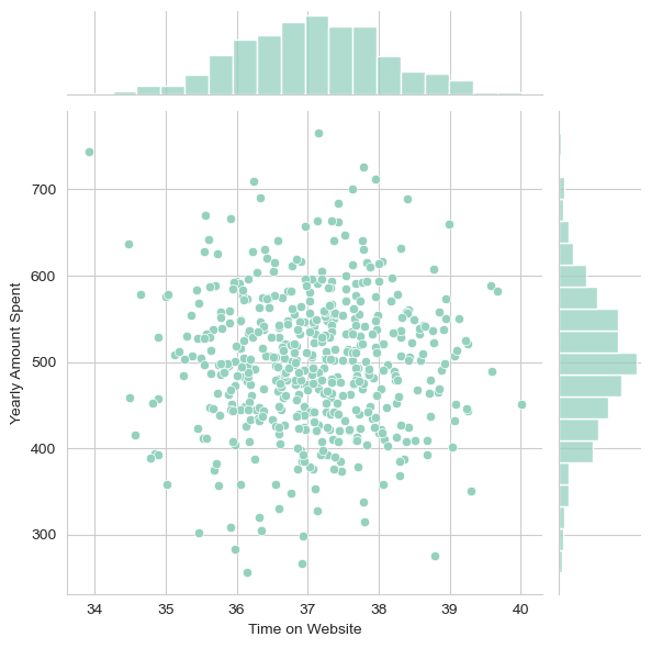
Conclusion: More time on site, more money spent.
sns.jointplot(x='Time on App',y='Yearly Amount Spent',data=customers)
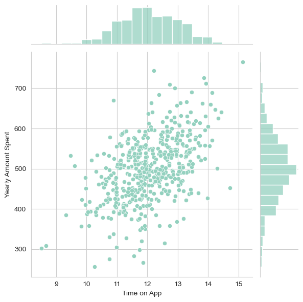
Conclusion: More time on App, more money spent.
sns.jointplot(x='Time on App',y='Length of Membership',data=customers)
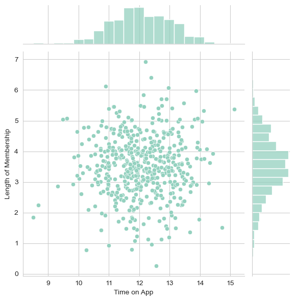
Conclusion: Positive correlation between length of membership and time on App.
sns.pairplot(customers)
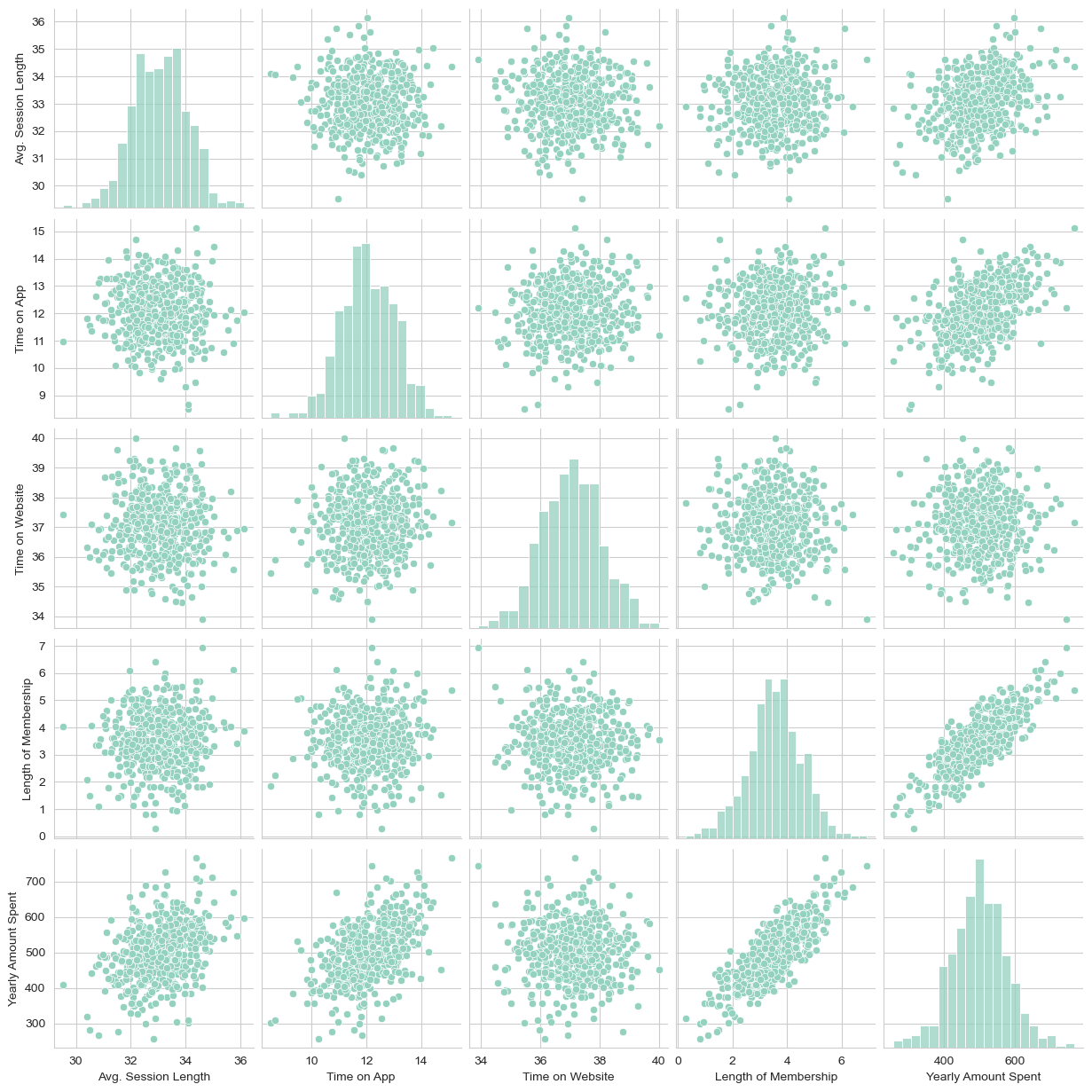
Based off this plot length of membership looks to be the most correlated feature with Yearly Amount Spent.
Split Input Variables and Output Variables
X = customers.drop(['Email', 'Address', 'Avatar', 'Yearly Amount Spent'], axis = 1)
y = customers['Yearly Amount Spent']
Split out Training and Test Sets
from sklearn.model_selection import train_test_split

X_train, X_test, y_train, y_test = train_test_split(X, y, test_size = 0.2, random_state = 42)
Model Training
from sklearn.linear_model import LinearRegression

regressor = LinearRegression()
regressor.fit(X_train, y_train)
Prediction on the Teat Set
y_predict = regressor.predict(X_test)
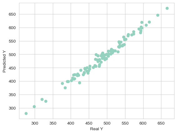
Model Assessment (Validation)
Creating a scatterplot of the real test values versus the predicted values
plt.scatter(y_test, y_predict)
plt.xlabel('Real Y')
plt.ylabel('Predicted Y')
Text(0, 0.5, 'Predicted Y')
Calculating the Mean Absolute Error, Mean Squared Error, and the Root Mean Squared Error
from sklearn import metrics

print('MAE:', metrics.mean_absolute_error(y_test, y_predict))
print('MSE:', metrics.mean_squared_error(y_test, y_predict))
print('RMSE:', np.sqrt(metrics.mean_squared_error(y_test, y_predict)))
MAE: 8.558441885315233
MSE: 109.86374118393995
RMSE: 10.481590584636473
Calculating R-squared
from sklearn.metrics import r2_score

r_squared = r2_score(y_test, y_predict)
print(r_squared)
0.9778130629184126
Extracting Model Coefficients
regressor.intercept_
-1044.2574146365582
regressor.coef_
array([25.5962591 , 38.78534598, 0.31038593, 61.89682859])
pd.DataFrame(regressor.coef_, X.columns, columns = ['Coefficents'])
| Coefficents | |
|---|---|
| Avg. Session Length | 25.596259 |
| Time on App | 38.785346 |
| Time on Website | 0.310386 |
| Length of Membership | 61.896829 |
Interpreting the coefficients:
- Holding all other features fixed, a 1 unit increase in Avg. Session Length is associated with an increase of 25.6 total dollars spent.
- Holding all other features fixed, a 1 unit increase in Time on App is associated with an increase of 38.8 total dollars spent.
- Holding all other features fixed, a 1 unit increase in Time on Website is associated with an increase of 0.3 total dollars spent.
- Holding all other features fixed, a 1 unit increase in Length of Membership is associated with an increase of 61.9 total dollars spent.