Predicting Loan Repayment- Analyzing LendingClub Data for Credit Risk Assessment
LendingClub is a US peer-to-peer lending company, headquartered in San Francisco, California[3]. It was the first peer-to-peer lender to register its offerings as securities with the Securities and Exchange Commission (SEC), and to offer loan trading on a secondary market. LendingClub is the world’s largest peer-to-peer lending platform.
I used a subset of the LendingClub DataSet obtained from Kaggle: https://www.kaggle.com/wordsforthewise/lending-club
Given historical data on loans given out with information on whether or not the borrower defaulted (charge-off), I built a model to predict whether or not a borrower would pay back their loan? This way in the future when we get a new potential customer we can assess whether or not they are likely to pay back the loan.
The “loan_status” column contains the label.
Data Overview
Here is the information on this particular data set:
| LoanStatNew | Description | |
|---|---|---|
| 0 | loan_amnt | The listed amount of the loan applied for by the borrower. If at some point in time, the credit department reduces the loan amount, then it will be reflected in this value. |
| 1 | term | The number of payments on the loan. Values are in months and can be either 36 or 60. |
| 2 | int_rate | Interest Rate on the loan |
| 3 | installment | The monthly payment owed by the borrower if the loan originates. |
| 4 | grade | LC assigned loan grade |
| 5 | sub_grade | LC assigned loan subgrade |
| 6 | emp_title | The job title supplied by the Borrower when applying for the loan.* |
| 7 | emp_length | Employment length in years. Possible values are between 0 and 10 where 0 means less than one year and 10 means ten or more years. |
| 8 | home_ownership | The home ownership status provided by the borrower during registration or obtained from the credit report. Our values are: RENT, OWN, MORTGAGE, OTHER |
| 9 | annual_inc | The self-reported annual income provided by the borrower during registration. |
| 10 | verification_status | Indicates if income was verified by LC, not verified, or if the income source was verified |
| 11 | issue_d | The month which the loan was funded |
| 12 | loan_status | Current status of the loan |
| 13 | purpose | A category provided by the borrower for the loan request. |
| 14 | title | The loan title provided by the borrower |
| 15 | zip_code | The first 3 numbers of the zip code provided by the borrower in the loan application. |
| 16 | addr_state | The state provided by the borrower in the loan application |
| 17 | dti | A ratio calculated using the borrower’s total monthly debt payments on the total debt obligations, excluding mortgage and the requested LC loan, divided by the borrower’s self-reported monthly income. |
| 18 | earliest_cr_line | The month the borrower's earliest reported credit line was opened |
| 19 | open_acc | The number of open credit lines in the borrower's credit file. |
| 20 | pub_rec | Number of derogatory public records |
| 21 | revol_bal | Total credit revolving balance |
| 22 | revol_util | Revolving line utilization rate, or the amount of credit the borrower is using relative to all available revolving credit. |
| 23 | total_acc | The total number of credit lines currently in the borrower's credit file |
| 24 | initial_list_status | The initial listing status of the loan. Possible values are – W, F |
| 25 | application_type | Indicates whether the loan is an individual application or a joint application with two co-borrowers |
| 26 | mort_acc | Number of mortgage accounts. |
| 27 | pub_rec_bankruptcies | Number of public record bankruptcies |
Import Required Packages and Data
import pandas as pd
import numpy as np
import matplotlib.pyplot as plt
import seaborn as sns
df = pd.read_csv('../DATA/lending_club_loan_two.csv')
df.info()
<class 'pandas.core.frame.DataFrame'>
RangeIndex: 396030 entries, 0 to 396029
Data columns (total 27 columns):
 #   Column                Non-Null Count   Dtype
---  ------                --------------   -----
 0   loan_amnt             396030 non-null  float64
 1   term                  396030 non-null  object
 2   int_rate              396030 non-null  float64
 3   installment           396030 non-null  float64
 4   grade                 396030 non-null  object
 5   sub_grade             396030 non-null  object
 6   emp_title             373103 non-null  object
 7   emp_length            377729 non-null  object
 8   home_ownership        396030 non-null  object
 9   annual_inc            396030 non-null  float64
 10  verification_status   396030 non-null  object
 11  issue_d               396030 non-null  object
 12  loan_status           396030 non-null  object
 13  purpose               396030 non-null  object
 14  title                 394275 non-null  object
 15  dti                   396030 non-null  float64
 16  earliest_cr_line      396030 non-null  object
 17  open_acc              396030 non-null  float64
 18  pub_rec               396030 non-null  float64
 19  revol_bal             396030 non-null  float64
 20  revol_util            395754 non-null  float64
 21  total_acc             396030 non-null  float64
 22  initial_list_status   396030 non-null  object
 23  application_type      396030 non-null  object
 24  mort_acc              358235 non-null  float64
 25  pub_rec_bankruptcies  395495 non-null  float64
 26  address               396030 non-null  object
dtypes: float64(12), object(15)
memory usage: 81.6+ MB
df.head()
| loan_amnt | term | int_rate | installment | grade | sub_grade | emp_title | emp_length | home_ownership | annual_inc | ... | open_acc | pub_rec | revol_bal | revol_util | total_acc | initial_list_status | application_type | mort_acc | pub_rec_bankruptcies | address | |
|---|---|---|---|---|---|---|---|---|---|---|---|---|---|---|---|---|---|---|---|---|---|
| 0 | 10000.0 | 36 months | 11.44 | 329.48 | B | B4 | Marketing | 10+ years | RENT | 117000.0 | ... | 16.0 | 0.0 | 36369.0 | 41.8 | 25.0 | w | INDIVIDUAL | 0.0 | 0.0 | 0174 Michelle Gateway\nMendozaberg, OK 22690 |
| 1 | 8000.0 | 36 months | 11.99 | 265.68 | B | B5 | Credit analyst | 4 years | MORTGAGE | 65000.0 | ... | 17.0 | 0.0 | 20131.0 | 53.3 | 27.0 | f | INDIVIDUAL | 3.0 | 0.0 | 1076 Carney Fort Apt. 347\nLoganmouth, SD 05113 |
| 2 | 15600.0 | 36 months | 10.49 | 506.97 | B | B3 | Statistician | < 1 year | RENT | 43057.0 | ... | 13.0 | 0.0 | 11987.0 | 92.2 | 26.0 | f | INDIVIDUAL | 0.0 | 0.0 | 87025 Mark Dale Apt. 269\nNew Sabrina, WV 05113 |
| 3 | 7200.0 | 36 months | 6.49 | 220.65 | A | A2 | Client Advocate | 6 years | RENT | 54000.0 | ... | 6.0 | 0.0 | 5472.0 | 21.5 | 13.0 | f | INDIVIDUAL | 0.0 | 0.0 | 823 Reid Ford\nDelacruzside, MA 00813 |
| 4 | 24375.0 | 60 months | 17.27 | 609.33 | C | C5 | Destiny Management Inc. | 9 years | MORTGAGE | 55000.0 | ... | 13.0 | 0.0 | 24584.0 | 69.8 | 43.0 | f | INDIVIDUAL | 1.0 | 0.0 | 679 Luna Roads\nGreggshire, VA 11650 |
5 rows × 27 columns
Part1: Exploratory Data Analysis
Since I wanted to predict loan_status, I created a countplot as shown below to see how balanced the labels were:
sns.countplot(x='loan_status', data=df)
<Axes: xlabel='loan_status', ylabel='count'>
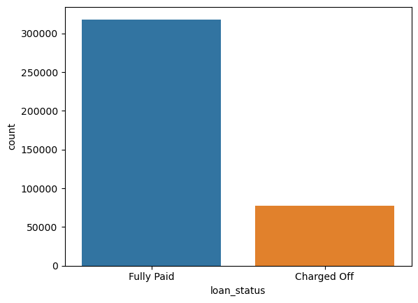
I had an imbalanced dataset. I expected to do very well in terms of accuracy but I had to use recall and precision to evaluate my data.
I created a histogram of the loan_amnt column.
plt.figure(figsize=(9,4))
sns.histplot(data=df,x='loan_amnt', bins=40)
<Axes: xlabel='loan_amnt', ylabel='Count'>
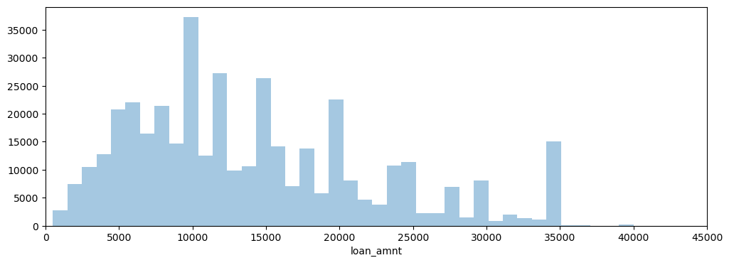
It showed that the vast majority of loans were between 5000 and 25000$.
I then explored correlation between the continuous feature variables and visualize it using heatmap.
df.corr()
| loan_amnt | int_rate | installment | annual_inc | dti | open_acc | pub_rec | revol_bal | revol_util | total_acc | mort_acc | pub_rec_bankruptcies | |
|---|---|---|---|---|---|---|---|---|---|---|---|---|
| loan_amnt | 1.000000 | 0.168921 | 0.953929 | 0.336887 | 0.016636 | 0.198556 | -0.077779 | 0.328320 | 0.099911 | 0.223886 | 0.222315 | -0.106539 |
| int_rate | 0.168921 | 1.000000 | 0.162758 | -0.056771 | 0.079038 | 0.011649 | 0.060986 | -0.011280 | 0.293659 | -0.036404 | -0.082583 | 0.057450 |
| installment | 0.953929 | 0.162758 | 1.000000 | 0.330381 | 0.015786 | 0.188973 | -0.067892 | 0.316455 | 0.123915 | 0.202430 | 0.193694 | -0.098628 |
| annual_inc | 0.336887 | -0.056771 | 0.330381 | 1.000000 | -0.081685 | 0.136150 | -0.013720 | 0.299773 | 0.027871 | 0.193023 | 0.236320 | -0.050162 |
| dti | 0.016636 | 0.079038 | 0.015786 | -0.081685 | 1.000000 | 0.136181 | -0.017639 | 0.063571 | 0.088375 | 0.102128 | -0.025439 | -0.014558 |
| open_acc | 0.198556 | 0.011649 | 0.188973 | 0.136150 | 0.136181 | 1.000000 | -0.018392 | 0.221192 | -0.131420 | 0.680728 | 0.109205 | -0.027732 |
| pub_rec | -0.077779 | 0.060986 | -0.067892 | -0.013720 | -0.017639 | -0.018392 | 1.000000 | -0.101664 | -0.075910 | 0.019723 | 0.011552 | 0.699408 |
| revol_bal | 0.328320 | -0.011280 | 0.316455 | 0.299773 | 0.063571 | 0.221192 | -0.101664 | 1.000000 | 0.226346 | 0.191616 | 0.194925 | -0.124532 |
| revol_util | 0.099911 | 0.293659 | 0.123915 | 0.027871 | 0.088375 | -0.131420 | -0.075910 | 0.226346 | 1.000000 | -0.104273 | 0.007514 | -0.086751 |
| total_acc | 0.223886 | -0.036404 | 0.202430 | 0.193023 | 0.102128 | 0.680728 | 0.019723 | 0.191616 | -0.104273 | 1.000000 | 0.381072 | 0.042035 |
| mort_acc | 0.222315 | -0.082583 | 0.193694 | 0.236320 | -0.025439 | 0.109205 | 0.011552 | 0.194925 | 0.007514 | 0.381072 | 1.000000 | 0.027239 |
| pub_rec_bankruptcies | -0.106539 | 0.057450 | -0.098628 | -0.050162 | -0.014558 | -0.027732 | 0.699408 | -0.124532 | -0.086751 | 0.042035 | 0.027239 | 1.000000 |
plt.figure(figsize=(9,6))
sns.heatmap(df.corr(), annot=True, cmap='YlGnBu')
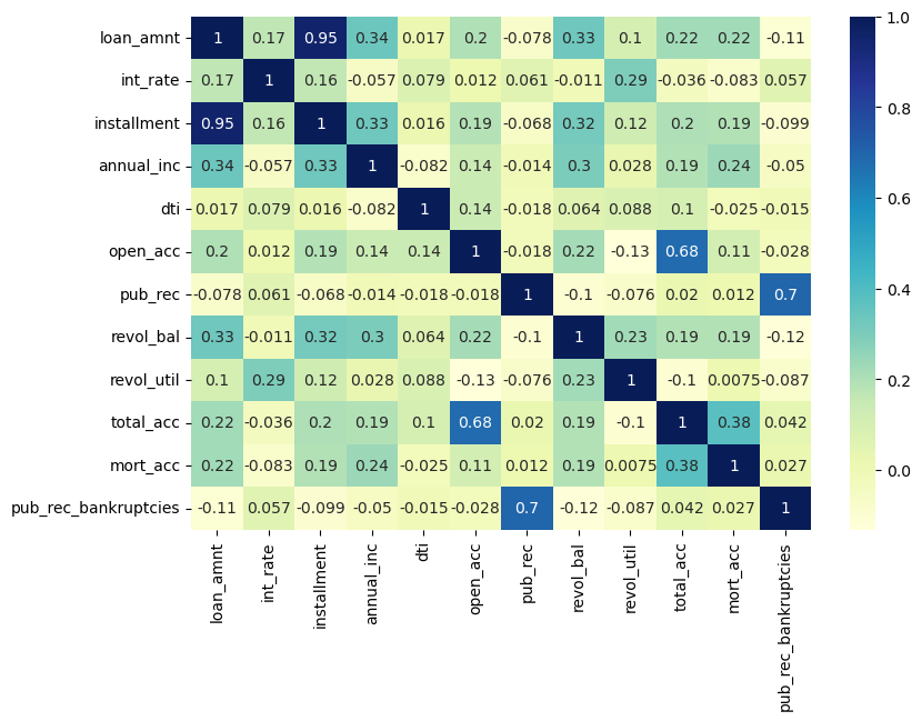
I noticed an almost perfect correlation between the loan amount and “installment” features and tried to explore these features further. For that, I first found their description and then drew a scatterplot between them.
data_info = pd.read_csv('../DATA/lending_club_info.csv',index_col='LoanStatNew')

def feature_info(col_name):
    print(data_info.loc[col_name]['Description'])
feature_info('installment')
The monthly payment owed by the borrower if the loan originates.
feature_info('loan_amnt')
The listed amount of the loan applied for by the borrower. If at some point in time, the credit department reduces the loan amount, then it will be reflected in this value.
sns.scatterplot(y='loan_amnt', x='installment', data=df)
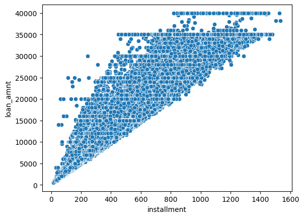
A perfect correlation was noticed between these two features.
I tried to see if there was any relationship between the loan status and the amount of the loan. For that, I created a boxplot.
sns.boxplot(data=df, x='loan_status', y='loan_amnt')
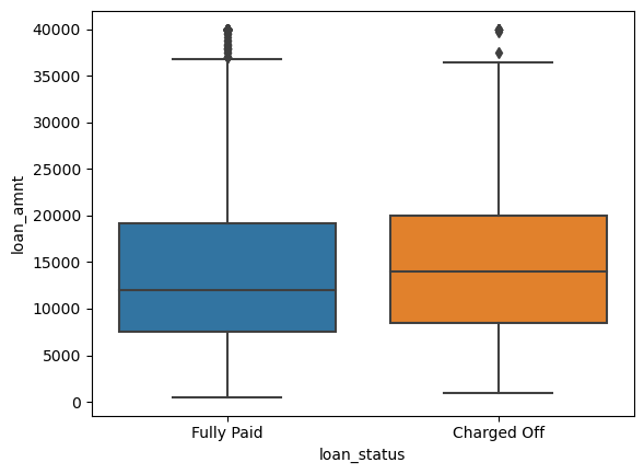
They looked pretty similar.
Then, I calculated the summary statistics for the loan amount, grouped by the loan_status.
df.groupby('loan_status')['loan_amnt'].describe()
| count | mean | std | min | 25% | 50% | 75% | max | |
|---|---|---|---|---|---|---|---|---|
| loan_status | ||||||||
| Charged Off | 77673.0 | 15126.300967 | 8505.090557 | 1000.0 | 8525.0 | 14000.0 | 20000.0 | 40000.0 |
| Fully Paid | 318357.0 | 13866.878771 | 8302.319699 | 500.0 | 7500.0 | 12000.0 | 19225.0 | 40000.0 |
The average loan amount of the charged-off group was a little higher than fully paid ones which made sense as higher loan amounts were more difficult to pay off.
I explored the Grade and SubGrade columns that LendingClub attributed to the loans and checked the unique possible grades and subgrades.
grade_order = sorted(df['grade'].unique())
Subgrade_order = sorted(df['sub_grade'].unique())
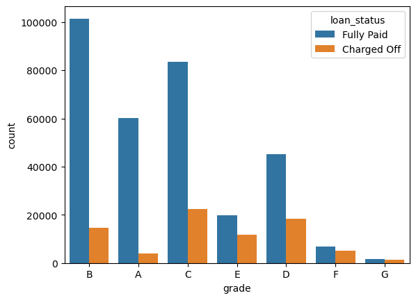
I created a countplot per grade to see the loan status . I set the hue to the loan_status label.
sns.countplot(x='grade', hue='loan_status', data=df)
<Axes: xlabel='grade', ylabel='count'>
I ordered the bars from grade A to E
sns.countplot(x='grade', hue='loan_status', data=df, order=grade_order)
<Axes: xlabel='grade', ylabel='count'>
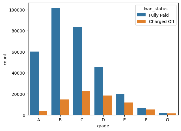
Moving from grade A to G, the ratio of fully paid loans to charged off loans decreased meaning that we faced riskier groups.
I drew a count plot per subgrade.
plt.figure(figsize=(10,4))
sns.countplot(x='sub_grade', data=df, order=Subgrade_order, palette='coolwarm')
<Axes: xlabel='sub_grade', ylabel='count'>
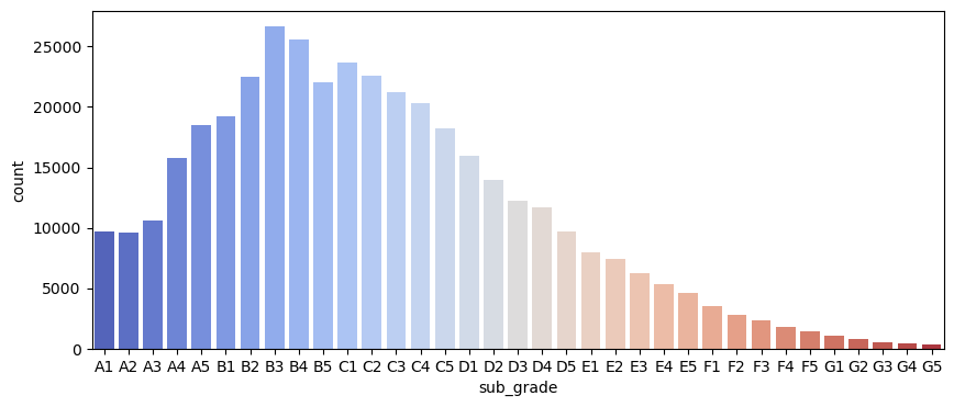
A decrease in the number of loans was seen when moving from sub_grades A to G which makde sense as we moved towards riskier groups.
Then, I checked all loans made per subgrade separated based on the loan_status.
plt.figure(figsize=(10,4))
sns.countplot(x='sub_grade', data=df, order=Subgrade_order, hue='loan_status', palette='coolwarm')
<Axes: xlabel='sub_grade', ylabel='count'>
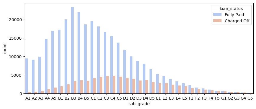
It looked like F and G subgrades didn’t get paid back that often. I isolated those and recreated the countplot just for those subgrades.
F_and_G = df[(df['grade']=='F')|(df['grade']=='G')]
F_and_G_sub_grade_order = sorted((F_and_G)['sub_grade'].unique())
plt.figure(figsize=(10,4))
sns.countplot(x='sub_grade', data=df, order=F_and_G_sub_grade_order, hue='loan_status', palette='coolwarm')
<Axes: xlabel='sub_grade', ylabel='count'>
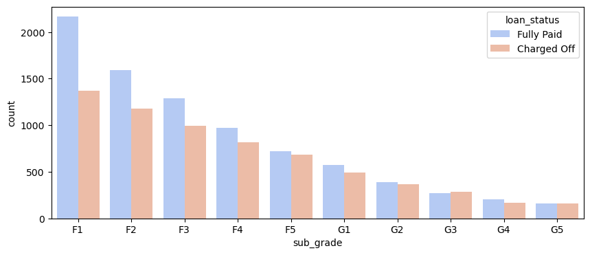
As shown in the above figure, the number of fully paid loans was almost equal to the number of charged-off ones for grades F and G.
Id create a new column called ‘loan_repaid’ which contained a 1 if the loan status was “Fully Paid” and a 0 if it was “Charged Off”.**
def status(x):
    if x=='Fully Paid':
        return 1
    else:
        return 0
df['loan_repaid'] = df['loan_status'].apply(status)
| loan_repaid | loan_status | |
|---|---|---|
| 0 | 1 | Fully Paid |
| 1 | 1 | Fully Paid |
| 2 | 1 | Fully Paid |
| 3 | 1 | Fully Paid |
| 4 | 0 | Charged Off |
| ... | ... | ... |
| 396025 | 1 | Fully Paid |
| 396026 | 1 | Fully Paid |
| 396027 | 1 | Fully Paid |
| 396028 | 1 | Fully Paid |
| 396029 | 1 | Fully Paid |
396030 rows × 2 columns
df.corr()['loan_repaid'].sort_values().drop('loan_repaid').plot(kind='bar')
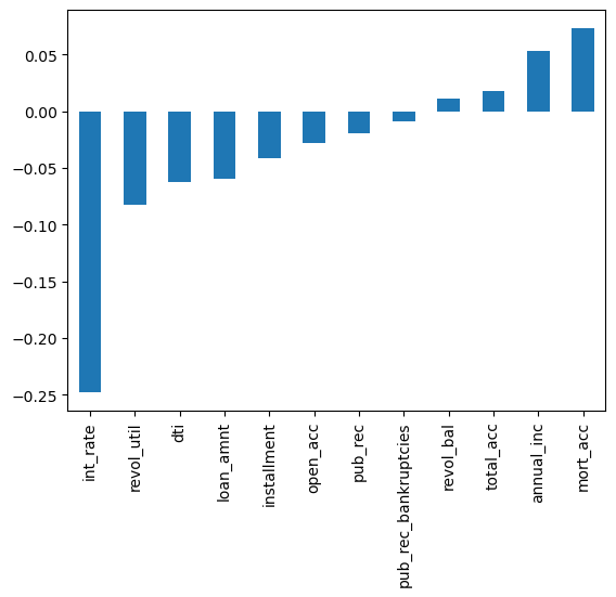
The interest rate had the highest negative correlation with loan_repaid which totally made sense as higher interest rate made it more difficult to repay the loan.
Part 2: Data PreProcessing
df.head()
| loan_amnt | term | int_rate | installment | grade | sub_grade | emp_title | emp_length | home_ownership | annual_inc | ... | pub_rec | revol_bal | revol_util | total_acc | initial_list_status | application_type | mort_acc | pub_rec_bankruptcies | address | loan_repaid | |
|---|---|---|---|---|---|---|---|---|---|---|---|---|---|---|---|---|---|---|---|---|---|
| 0 | 10000.0 | 36 months | 11.44 | 329.48 | B | B4 | Marketing | 10+ years | RENT | 117000.0 | ... | 0.0 | 36369.0 | 41.8 | 25.0 | w | INDIVIDUAL | 0.0 | 0.0 | 0174 Michelle Gateway\nMendozaberg, OK 22690 | 1 |
| 1 | 8000.0 | 36 months | 11.99 | 265.68 | B | B5 | Credit analyst | 4 years | MORTGAGE | 65000.0 | ... | 0.0 | 20131.0 | 53.3 | 27.0 | f | INDIVIDUAL | 3.0 | 0.0 | 1076 Carney Fort Apt. 347\nLoganmouth, SD 05113 | 1 |
| 2 | 15600.0 | 36 months | 10.49 | 506.97 | B | B3 | Statistician | < 1 year | RENT | 43057.0 | ... | 0.0 | 11987.0 | 92.2 | 26.0 | f | INDIVIDUAL | 0.0 | 0.0 | 87025 Mark Dale Apt. 269\nNew Sabrina, WV 05113 | 1 |
| 3 | 7200.0 | 36 months | 6.49 | 220.65 | A | A2 | Client Advocate | 6 years | RENT | 54000.0 | ... | 0.0 | 5472.0 | 21.5 | 13.0 | f | INDIVIDUAL | 0.0 | 0.0 | 823 Reid Ford\nDelacruzside, MA 00813 | 1 |
| 4 | 24375.0 | 60 months | 17.27 | 609.33 | C | C5 | Destiny Management Inc. | 9 years | MORTGAGE | 55000.0 | ... | 0.0 | 24584.0 | 69.8 | 43.0 | f | INDIVIDUAL | 1.0 | 0.0 | 679 Luna Roads\nGreggshire, VA 11650 | 0 |
5 rows × 28 columns
Missing Data
I used a variety of factors to decide whether or not they would be useful, and to see if I should keep, discard, or fill in the missing data.
Length of the dataframe:
df_length = len(df)
Total count of missing values per column:
df.isna().sum()
loan_amnt                   0
term                        0
int_rate                    0
installment                 0
grade                       0
sub_grade                   0
emp_title               22927
emp_length              18301
home_ownership              0
annual_inc                  0
verification_status         0
issue_d                     0
loan_status                 0
purpose                     0
title                    1755
dti                         0
earliest_cr_line            0
open_acc                    0
pub_rec                     0
revol_bal                   0
revol_util                276
total_acc                   0
initial_list_status         0
application_type            0
mort_acc                37795
pub_rec_bankruptcies      535
address                     0
loan_repaid                 0
dtype: int64
Total percentage of missing values per column:
df.isna().sum()/(df_length)*100
loan_amnt               0.000000
term                    0.000000
int_rate                0.000000
installment             0.000000
grade                   0.000000
sub_grade               0.000000
emp_title               5.789208
emp_length              4.621115
home_ownership          0.000000
annual_inc              0.000000
verification_status     0.000000
issue_d                 0.000000
loan_status             0.000000
purpose                 0.000000
title                   0.443148
dti                     0.000000
earliest_cr_line        0.000000
open_acc                0.000000
pub_rec                 0.000000
revol_bal               0.000000
revol_util              0.069692
total_acc               0.000000
initial_list_status     0.000000
application_type        0.000000
mort_acc                9.543469
pub_rec_bankruptcies    0.135091
address                 0.000000
loan_repaid             0.000000
dtype: float64
I examined emp_title and emp_length to see whether it would be okay to drop them.
feature_info('emp_title')
The job title supplied by the Borrower when applying for the loan.
feature_info('emp_length')
Employment length in years. Possible values were between 0 and 10 where 0 meant less than one year and 10 meant ten or more years.
Number of unique employment job titles:
df['emp_title'].nunique()
173105
df['emp_title'].value_counts()
Teacher                    4389
Manager                    4250
Registered Nurse           1856
RN                         1846
Supervisor                 1830
                           ...
Postman                       1
McCarthy & Holthus, LLC       1
jp flooring                   1
Histology Technologist        1
Gracon Services, Inc          1
Name: emp_title, Length: 173105, dtype: int64
Realistically there were too many unique job titles to try to convert to numeric feature. Therefore, I removed that emp_title column.
df = df.drop('emp_title', axis=1)
I created a count plot of the emp_length feature column, sorted by the order of the values.
df['emp_length'].dropna().unique()
['1 year',
 '10+ years',
 '2 years',
 '3 years',
 '4 years',
 '5 years',
 '6 years',
 '7 years',
 '8 years',
 '9 years',
 '< 1 year']
emp_length_order = sorted(df['emp_length'].dropna().unique())
emp_length_order = [ ‘< 1 year’, ‘1 year’, ‘2 years’, ‘3 years’, ‘4 years’, ‘5 years’, ‘6 years’, ‘7 years’, ‘8 years’, ‘9 years’, ‘10+ years’]
```python
plt.figure(figsize=(10,4))
sns.countplot(data=df, x='emp_length', order=emp_length_order)
It seemed that the majority of people who took loan had been working for more than 10 years which made sense as I had to have a kind of job security to be able to repay the loan.
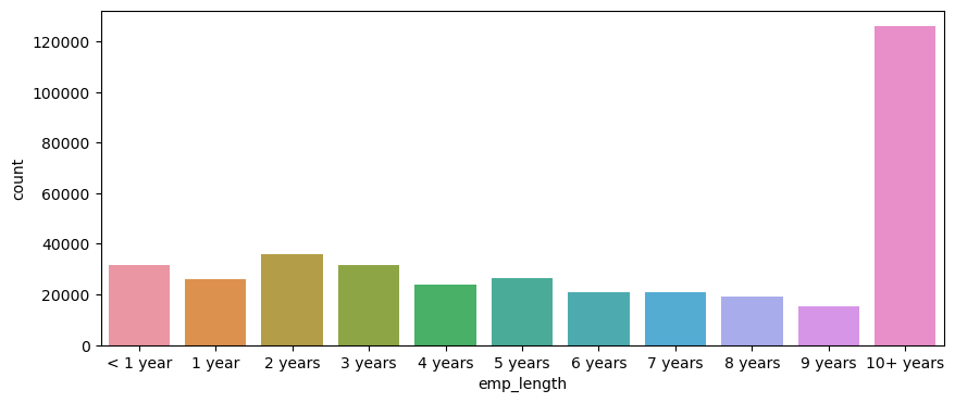
I plotted out the countplot with a hue separating Fully Paid vs Charged Off
plt.figure(figsize=(10,4))
sns.countplot(data=df, x='emp_length', order=emp_length_order, hue= 'loan_status')
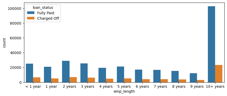
For people with more than 10+ years of employment length, the number of fully paid loans was much higher than charged-off ones.
I found the percentage of charge-offs per category to see what percent of people per employment category didn’t pay back their loan. It might help me to understand if there was a strong relationship between employment length and being charged off.
fully_paid_number = df[df['loan_status']=='Fully Paid'].groupby('emp_length').count()['loan_status']
charged_off_number = df[df['loan_status']=='Charged Off'].groupby('emp_length').count()['loan_status']
total_loan_number = fully_paid_number + charged_off_number
charged_off_percentage = charged_off_number/total_loan_number*100
plt.figure(figsize=(8,4))
charged_off_percentage.plot(kind='bar')
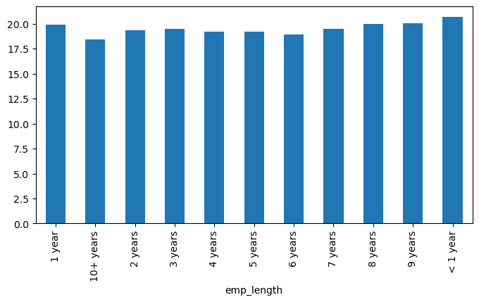
Charge off rates were similar across all employment lengths.
Then, I dropped the emp_length column.
df = df.drop('emp_length', axis=1)
I revisited the DataFrame to see what feature columns still had missing data.
df.isna().sum()
loan_amnt                   0
term                        0
int_rate                    0
installment                 0
grade                       0
sub_grade                   0
home_ownership              0
annual_inc                  0
verification_status         0
issue_d                     0
loan_status                 0
purpose                     0
title                    1755
dti                         0
earliest_cr_line            0
open_acc                    0
pub_rec                     0
revol_bal                   0
revol_util                276
total_acc                   0
initial_list_status         0
application_type            0
mort_acc                37795
pub_rec_bankruptcies      535
address                     0
loan_repaid                 0
dtype: int64
Then I reviewed the title column vs the purpose column to see if there was any repeated information.
df['purpose'].head(10)
0              vacation
1    debt_consolidation
2           credit_card
3           credit_card
4           credit_card
5    debt_consolidation
6      home_improvement
7           credit_card
8    debt_consolidation
9    debt_consolidation
Name: purpose, dtype: object
df['title'].head(10)
0                   Vacation
1         Debt consolidation
2    Credit card refinancing
3    Credit card refinancing
4      Credit Card Refinance
5         Debt consolidation
6           Home improvement
7       No More Credit Cards
8         Debt consolidation
9         Debt Consolidation
Name: title, dtype: object
It seemed that the title column was simply a string subcategory/description of the purpose column. Therefore, I dropped the title column.
df = df.drop('title', axis=1)
I tried to find out what the mort_acc feature represented.
feature_info('mort_acc')
Number of mortgage accounts.
I created a value_counts of the mort_acc column.
df['mort_acc'].value_counts()
0.0     139777
1.0      60416
2.0      49948
3.0      38049
4.0      27887
5.0      18194
6.0      11069
7.0       6052
8.0       3121
9.0       1656
10.0       865
11.0       479
12.0       264
13.0       146
14.0       107
15.0        61
16.0        37
17.0        22
18.0        18
19.0        15
20.0        13
24.0        10
22.0         7
21.0         4
25.0         4
27.0         3
32.0         2
31.0         2
23.0         2
26.0         2
28.0         1
30.0         1
34.0         1
Name: mort_acc, dtype: int64
Then, I reviewed the other columns to see which most highly correlates to mort_acc.
df.corr()['mort_acc'].sort_values()
int_rate               -0.082583
dti                    -0.025439
revol_util              0.007514
pub_rec                 0.011552
pub_rec_bankruptcies    0.027239
loan_repaid             0.073111
open_acc                0.109205
installment             0.193694
revol_bal               0.194925
loan_amnt               0.222315
annual_inc              0.236320
total_acc               0.381072
mort_acc                1.000000
Name: mort_acc, dtype: float64
I Looked like the total_acc feature correlated with the mort_acc , this made sense!
feature_info('total_acc')
The total number of credit lines currently in the borrower's credit file
I tried the fillna() approach to replace missing data. I grouped the dataframe by the total_acc and calculated the mean value for the mort_acc per total_acc entry.
df_acc = df[['total_acc','mort_acc']].sort_values(by='total_acc')
df_acc
mort_acc_mean = df.groupby('total_acc')['mort_acc'].mean()
I filled in the missing mort_acc values based on their total_acc value. If the mort_acc was missing, then I filled in that missing value with the mean value corresponding to its total_acc value.
mort_acc_mean = pd.DataFrame(mort_acc_mean)
mort_acc_mean.columns = ['mort_acc_mean']
df_acc = df_acc.merge(mort_acc_mean, on='total_acc', how='inner')
df['mort_acc'].fillna(value=df_acc['mort_acc_mean'], inplace=True)
df.isna().sum()
revol_util and the pub_rec_bankruptcies had missing data points, but they accounted for less than 0.5% of the total data. Therefore, I removed the rows that were missing those values in those columns.
df = df.dropna()
df.isna().sum()
loan_amnt                   0
term                        0
int_rate                    0
installment                 0
grade                       0
sub_grade                   0
home_ownership              0
annual_inc                  0
verification_status         0
issue_d                     0
loan_status                 0
purpose                     0
dti                         0
earliest_cr_line            0
open_acc                    0
pub_rec                     0
revol_bal                   0
revol_util                276
total_acc                   0
initial_list_status         0
application_type            0
mort_acc                37795
pub_rec_bankruptcies      535
address                     0
loan_repaid                 0
dtype: int64
Categorical Variables
Here, I Listed all the columns that were non-numeric.
df.select_dtypes(['object']).columns
Index(['term', 'grade', 'sub_grade', 'home_ownership', 'verification_status',
       'issue_d', 'loan_status', 'purpose', 'earliest_cr_line',
       'initial_list_status', 'application_type', 'address'],
      dtype='object')
term feature
df['term'].value_counts()
 36 months    302005
 60 months     94025
Name: term, dtype: int64
term feature had just 2 values of 36 and 60 months. I removed the month and simply converted the categorical data to numeric one.
def  conversion(x):
    return int(x[1:3])

df['term'] = df['term'].apply(conversion)
# Alternative: df['term'] = df['term'].apply(lambda term: int(term[:3]))
df['term'].value_counts()
36    302005
60     94025
Name: term, dtype: int64
grade feature: I already knew grade was part of sub_grade, so I dropped the grade feature.
df = df.drop('grade', axis=1)
sub_grade feature: I kept it to convert it to a numeric feature later on.
home_ownership feature:
df['home_ownership'].value_counts()
MORTGAGE    198348
RENT        159790
OWN          37746
OTHER          112
NONE            31
ANY              3
Name: home_ownership, dtype: int64
df['verification_status'].value_counts()
Verified           139563
Source Verified    131385
Not Verified       125082
Name: verification_status, dtype: int64
issue_d feature
df['issue_d'].value_counts()
Oct-2014    14846
Jul-2014    12609
Jan-2015    11705
Dec-2013    10618
Nov-2013    10496
            ...
Jul-2007       26
Sep-2008       25
Nov-2007       22
Sep-2007       15
Jun-2007        1
Name: issue_d, Length: 115, dtype: int64
This was data leakage as I wouldn’t know beforehand whether or not a loan would be issued when using my model, so in theory, I wouldn’t have an issue_date. I dropped this feature.
df = df = df.drop('issue_d', axis=1)
loan_status feature: As loan_status column was a duplicate of the loan_repaid column, I dropped the load_status column and used the loan_repaid column since its already in 0s and 1s.
df = df.drop('loan_status', axis=1)
purpose feature
df['purpose'].value_counts()
debt_consolidation    234507
credit_card            83019
home_improvement       24030
other                  21185
major_purchase          8790
small_business          5701
car                     4697
medical                 4196
moving                  2854
vacation                2452
house                   2201
wedding                 1812
renewable_energy         329
educational              257
Name: purpose, dtype: int64
earliest_cr_line feature
df['earliest_cr_line'].value_counts()
Oct-2000    3017
Aug-2000    2935
Oct-2001    2896
Aug-2001    2884
Nov-2000    2736
            ...
Jul-1958       1
Nov-1957       1
Jan-1953       1
Jul-1955       1
Aug-1959       1
Name: earliest_cr_line, Length: 684, dtype: int64
This appeareds to be a historical time stamp feature. I extracted the year from this feature and converted it to a numeric feature.
def year(x):
    return int(x[4:])

df['earliest_cr_line'].apply(year)
0         1990
1         2004
2         2007
3         2006
4         1999
          ...
396025    2004
396026    2006
396027    1997
396028    1990
396029    1998
Name: earliest_cr_line, Length: 396030, dtype: int64
I set this new data to a feature column called ‘earliest_cr_year’.Then dropped the earliest_cr_line feature.
df['earliest_cr_year']= df['earliest_cr_line'].apply(year)
df = df.drop('earliest_cr_line', axis=1)
initial_list_status feature
df['initial_list_status'].value_counts()
f    238066
w    157964
Name: initial_list_status, dtype: int64
application_type feature
df['application_type'].value_counts()
INDIVIDUAL    395319
JOINT            425
DIRECT_PAY       286
Name: application_type, dtype: int64
address feature
df['address'].value_counts()
USCGC Smith\nFPO AE 70466                           8
USS Johnson\nFPO AE 48052                           8
USNS Johnson\nFPO AE 05113                          8
USS Smith\nFPO AP 70466                             8
USNS Johnson\nFPO AP 48052                          7
                                                   ..
455 Tricia Cove\nAustinbury, FL 00813               1
7776 Flores Fall\nFernandezshire, UT 05113          1
6577 Mia Harbors Apt. 171\nRobertshire, OK 22690    1
8141 Cox Greens Suite 186\nMadisonstad, VT 05113    1
787 Michelle Causeway\nBriannaton, AR 48052         1
Name: address, Length: 393700, dtype: int64
I extracted the zip_code from address.
def zip_code(x):
    return x[-5:]

df ['zip_code'] = df['address'].apply(zip_code)
I dropped address column.
df = df.drop('address', axis=1)
Applying OneHotEncoder to convert all categorical features except loan_status to numeric ones.
from sklearn.preprocessing import OneHotEncoder

# Create a list of categorical variables
categorical_vars = ['sub_grade', 'home_ownership', 'verification_status',
       'purpose', 'initial_list_status', 'application_type', 'zip_code']

# Create and apply OneHotEncoder while removing the dummy variable
one_hot_encoder = OneHotEncoder(sparse = False, drop = 'first')

# Apply fit_transform on data
df_encoded = one_hot_encoder.fit_transform(df[categorical_vars])

# Get feature names to see what each column in the 'encoder_vars_array' presents
encoder_feature_names = one_hot_encoder.get_feature_names_out(categorical_vars)

# Convert our result from an array to a DataFrame
df_encoded = pd.DataFrame(df_encoded, columns = encoder_feature_names)

# Concatenate (Link together in a series or chain) new DataFrame to our original DataFrame
df = pd.concat([df.reset_index(drop = True),df_encoded.reset_index(drop = True)], axis = 1)

# Drop the original categorical variable columns
df.drop(categorical_vars, axis = 1, inplace = True)
Training Test Split
from sklearn.model_selection import train_test_split
Creating input and output variables
X = df.drop('loan_repaid', axis=1)
y = df['loan_repaid']
Due to low RAM, I grabbed a sample for data training to save time on training.
df = df.sample(frac=0.1,random_state=101)
print(len(df))
39603
X_train, X_test, y_train, y_test = train_test_split(X, y, test_size=0.20, random_state=101)
Normalizing the Data
from sklearn.preprocessing import MinMaxScaler

scaler = MinMaxScaler()
X_train = pd.DataFrame(scaler.fit_transform(X_train))
X_test = pd.DataFrame(scaler.transform(X_test))
Creating the Model
import tensorflow as tf
from tensorflow.keras.models import Sequential
from tensorflow.keras.layers import Dense,Dropout
X_train.shape
(316824, 80)
model = Sequential()

# input layer
model.add(Dense(80, activation='relu'))
model.add(Dropout(0.2))

# hidden layer
model.add(Dense(40, activation='relu'))
model.add(Dropout(0.2))

# hidden layer
model.add(Dense(20, activation='relu'))
model.add(Dropout(0.2))

# output layer
model.add(Dense(units=1,activation='sigmoid'))                       # output is either 0 or 1

# Compile model
model.compile(loss='binary_crossentropy', optimizer='adam')
fitting the model to the training data
model.fit(x=X_train,
          y=y_train,
          epochs=50,
          batch_size=256,
          validation_data=(X_test, y_test))
Epoch 1/50
[1238/1238 ━━━━━━━━━━━━━━━━━━━━  6ms/step - loss: 0.5360 - val_loss: 0.4944
Epoch 2/50
[1238/1238 ━━━━━━━━━━━━━━━━━━━━  5ms/step - loss: 0.4998 - val_loss: 0.4945
Epoch 3/50
[1238/1238 ━━━━━━━━━━━━━━━━━━━━  6ms/step - loss: 0.4974 - val_loss: 0.4944
Epoch 4/50
[1238/1238 ━━━━━━━━━━━━━━━━━━━━  6ms/step - loss: 0.4957 - val_loss: 0.4944
Epoch 5/50
[1238/1238 ━━━━━━━━━━━━━━━━━━━━  6ms/step - loss: 0.4973 - val_loss: 0.4943
Epoch 6/50
[1238/1238 ━━━━━━━━━━━━━━━━━━━━  6ms/step - loss: 0.4949 - val_loss: 0.4943
Epoch 7/50
[1238/1238 ━━━━━━━━━━━━━━━━━━━━  6ms/step - loss: 0.4948 - val_loss: 0.4943
Epoch 8/50
[1238/1238 ━━━━━━━━━━━━━━━━━━━━  5ms/step - loss: 0.4953 - val_loss: 0.4943
Epoch 9/50
[1238/1238 ━━━━━━━━━━━━━━━━━━━━  4ms/step - loss: 0.4959 - val_loss: 0.4943
Epoch 10/50
[1238/1238 ━━━━━━━━━━━━━━━━━━━━  5ms/step - loss: 0.4969 - val_loss: 0.4943
Epoch 11/50
[1238/1238 ━━━━━━━━━━━━━━━━━━━━  6ms/step - loss: 0.4947 - val_loss: 0.4944
Epoch 12/50
[1238/1238 ━━━━━━━━━━━━━━━━━━━━  6ms/step - loss: 0.4950 - val_loss: 0.4943
Epoch 13/50
[1238/1238 ━━━━━━━━━━━━━━━━━━━━  6ms/step - loss: 0.4960 - val_loss: 0.4944
Epoch 14/50
[1238/1238 ━━━━━━━━━━━━━━━━━━━━  6ms/step - loss: 0.4931 - val_loss: 0.4944
Epoch 15/50
[1238/1238 ━━━━━━━━━━━━━━━━━━━━  6ms/step - loss: 0.4938 - val_loss: 0.4943
Epoch 16/50
[1238/1238 ━━━━━━━━━━━━━━━━━━━━  4ms/step - loss: 0.4952 - val_loss: 0.4943
Epoch 17/50
[1238/1238 ━━━━━━━━━━━━━━━━━━━━  5ms/step - loss: 0.4964 - val_loss: 0.4944
Epoch 18/50
[1238/1238 ━━━━━━━━━━━━━━━━━━━━  5ms/step - loss: 0.4949 - val_loss: 0.4943
Epoch 19/50
[1238/1238 ━━━━━━━━━━━━━━━━━━━━  6ms/step - loss: 0.4961 - val_loss: 0.4943
Epoch 20/50
[1238/1238 ━━━━━━━━━━━━━━━━━━━━  6ms/step - loss: 0.4952 - val_loss: 0.4944
Epoch 21/50
[1238/1238 ━━━━━━━━━━━━━━━━━━━━  4ms/step - loss: 0.4939 - val_loss: 0.4943
Epoch 22/50
[1238/1238 ━━━━━━━━━━━━━━━━━━━━  4ms/step - loss: 0.4946 - val_loss: 0.4943
Epoch 23/50
[1238/1238 ━━━━━━━━━━━━━━━━━━━━  6ms/step - loss: 0.4957 - val_loss: 0.4943
Epoch 24/50
[1238/1238 ━━━━━━━━━━━━━━━━━━━━  6ms/step - loss: 0.4950 - val_loss: 0.4943
Epoch 25/50
[1238/1238 ━━━━━━━━━━━━━━━━━━━━  6ms/step - loss: 0.4956 - val_loss: 0.4943
Epoch 26/50
[1238/1238 ━━━━━━━━━━━━━━━━━━━━  6ms/step - loss: 0.4947 - val_loss: 0.4943
Epoch 27/50
[1238/1238 ━━━━━━━━━━━━━━━━━━━━  5ms/step - loss: 0.4937 - val_loss: 0.4943
Epoch 28/50
[1238/1238 ━━━━━━━━━━━━━━━━━━━━  5ms/step - loss: 0.4966 - val_loss: 0.4943
Epoch 29/50
[1238/1238 ━━━━━━━━━━━━━━━━━━━━  6ms/step - loss: 0.4954 - val_loss: 0.4943
Epoch 30/50
[1238/1238 ━━━━━━━━━━━━━━━━━━━━  5ms/step - loss: 0.4951 - val_loss: 0.4943
Epoch 31/50
[1238/1238 ━━━━━━━━━━━━━━━━━━━━  5ms/step - loss: 0.4955 - val_loss: 0.4943
Epoch 32/50
[1238/1238 ━━━━━━━━━━━━━━━━━━━━  5ms/step - loss: 0.4946 - val_loss: 0.4943
Epoch 33/50
[1238/1238 ━━━━━━━━━━━━━━━━━━━━  6ms/step - loss: 0.4950 - val_loss: 0.4943
Epoch 34/50
[1238/1238 ━━━━━━━━━━━━━━━━━━━━  6ms/step - loss: 0.4961 - val_loss: 0.4943
Epoch 35/50
[1238/1238 ━━━━━━━━━━━━━━━━━━━━  5ms/step - loss: 0.4952 - val_loss: 0.4943
Epoch 36/50
[1238/1238 ━━━━━━━━━━━━━━━━━━━━  4ms/step - loss: 0.4961 - val_loss: 0.4943
Epoch 37/50
[1238/1238 ━━━━━━━━━━━━━━━━━━━━  6ms/step - loss: 0.4957 - val_loss: 0.4943
Epoch 38/50
[1238/1238 ━━━━━━━━━━━━━━━━━━━━  6ms/step - loss: 0.4954 - val_loss: 0.4943
Epoch 39/50
[1238/1238 ━━━━━━━━━━━━━━━━━━━━  6ms/step - loss: 0.4967 - val_loss: 0.4943
Epoch 40/50
[1238/1238 ━━━━━━━━━━━━━━━━━━━━  6ms/step - loss: 0.4948 - val_loss: 0.4943
Epoch 41/50
[1238/1238 ━━━━━━━━━━━━━━━━━━━━  6ms/step - loss: 0.4942 - val_loss: 0.4943
Epoch 42/50
[1238/1238 ━━━━━━━━━━━━━━━━━━━━  6ms/step - loss: 0.4956 - val_loss: 0.4943
Epoch 43/50
[1238/1238 ━━━━━━━━━━━━━━━━━━━━  6ms/step - loss: 0.4939 - val_loss: 0.4944
Epoch 44/50
[1238/1238 ━━━━━━━━━━━━━━━━━━━━  6ms/step - loss: 0.4953 - val_loss: 0.4943
Epoch 45/50
[1238/1238 ━━━━━━━━━━━━━━━━━━━━  5ms/step - loss: 0.4942 - val_loss: 0.4943
Epoch 46/50
[1238/1238 ━━━━━━━━━━━━━━━━━━━━  6ms/step - loss: 0.4963 - val_loss: 0.4943
Epoch 47/50
[1238/1238 ━━━━━━━━━━━━━━━━━━━━  5ms/step - loss: 0.4962 - val_loss: 0.4943
Epoch 48/50
[1238/1238 ━━━━━━━━━━━━━━━━━━━━  5ms/step - loss: 0.4957 - val_loss: 0.4943
Epoch 49/50
[1238/1238 ━━━━━━━━━━━━━━━━━━━━  5ms/step - loss: 0.4966 - val_loss: 0.4944
Epoch 50/50
[1238/1238 ━━━━━━━━━━━━━━━━━━━━  6ms/step - loss: 0.4955 - val_loss: 0.4943
saving my model
from tensorflow.keras.models import load_model
model.save('full_data_project_model.h5')
Part 3: Evaluating Model Performance
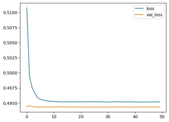
I plotted out the validation loss versus the training loss
loss = pd.DataFrame(model.history.history)
loss.plot()
<Axes: >
I created my our prediction from the X_test set and displayed a classification report and confusion matrix for the X_test set.
y_predict = model.predict(X_test)
y_predict
2476/2476 ━━━━━━━━━━━━━━━━━━━━ 6s 2ms/step
y_predict = pd.DataFrame(model.predict(X_test), columns=['Predicted Y'])
def p_class(x):
    if x>0.5:
        return 1
    else:
        return 0

y_predict_class = y_predict['Predicted Y'].apply(p_class)
y_predict_class
0        1
1        1
2        1
3        1
4        1
        ..
79201    1
79202    1
79203    1
79204    1
79205    1
Name: Predicted Y, Length: 79206, dtype: int64
from sklearn.metrics import classification_report,confusion_matrix
print(classification_report(y_test, y_predict_class))
              precision    recall  f1-score   support

           0       0.00      0.00      0.00     15493
           1       0.80      1.00      0.89     63713

    accuracy                           0.80     79206
   macro avg       0.40      0.50      0.45     79206
weighted avg       0.65      0.80      0.72     79206
confusion_matrix(y_test, y_predict_class)
array([[    0, 15493],
       [    0, 63713]], dtype=int64)
Part 4: New Case
Given the customer below, would you offer this person a loan?
import random
random.seed(101)
random_ind = random.randint(0,len(df))

new_customer = df.drop('loan_repaid',axis=1).iloc[random_ind]
new_customer
loan_amnt          2000.00
term                 36.00
int_rate              7.90
installment          62.59
annual_inc        20400.00
                    ...
zip_code_30723        0.00
zip_code_48052        0.00
zip_code_70466        0.00
zip_code_86630        1.00
zip_code_93700        0.00
Name: 87921, Length: 80, dtype: float64
I had to make sure that my data was numpy array not a dataframe.
new_customer = new_customer.values.reshape(1,80)
new_customer = scaler.transform(new_customer)
y_predict = model.predict(new_customer)
y_predict
1/1 ━━━━━━━━━━━━━━━━━━━━ 0s 40ms/step
y_predict = pd.DataFrame(model.predict(new_customer), columns=['Predicted Y'])
def p_class(x):
    if x>0.5:
        return 1
    else:
        return 0

y_predict_class = y_predict['Predicted Y'].apply(p_class)
y_predict_class
0    1
Name: Predicted Y, dtype: int64
I would probably give the loan to this person according to this model prediction.
Here, I checked if this person actually ended up paying back their loan.
df['loan_repaid'].iloc[random_ind]
0
It seemed that the customer had not actually repaid the loan.