Movie Recommendation System- Finding Similar Movies

5 minute read

In this project, we will focus on providing a basic recommendation system by suggesting items that are most similar to a particular item, in this case, movies. It tells us what movies/items are most similar to our movie choice.

Let’s get started!

Import Libraries

import numpy as np
import pandas as pd

Get the Data

column_names = ['user_id', 'item_id', 'rating', 'timestamp']
df = pd.read_csv('u.data', sep='\t', names=column_names)

df.head()

	user_id	item_id	rating	timestamp
0	0	50	5	881250949
1	0	172	5	881250949
2	0	133	1	881250949
3	196	242	3	881250949
4	186	302	3	891717742

Now let’s get the movie titles:

movie_titles = pd.read_csv("Movie_Id_Titles")
movie_titles.head()

	item_id	title
0	1	Toy Story (1995)
1	2	GoldenEye (1995)
2	3	Four Rooms (1995)
3	4	Get Shorty (1995)
4	5	Copycat (1995)

We can merge them together:

df = pd.merge(df,movie_titles,on='item_id')
df.head()

	user_id	item_id	rating	timestamp	title
0	0	50	5	881250949	Star Wars (1977)
1	290	50	5	880473582	Star Wars (1977)
2	79	50	4	891271545	Star Wars (1977)
3	2	50	5	888552084	Star Wars (1977)
4	8	50	5	879362124	Star Wars (1977)

EDA

Let’s explore the data a bit and get a look at some of the best rated movies.

Visualization Imports

import matplotlib.pyplot as plt
import seaborn as sns
sns.set_style('white')
%matplotlib inline

Let’s create a ratings dataframe with average rating and number of ratings:

df.groupby('title')['rating'].mean().sort_values(ascending=False).head()

title
They Made Me a Criminal (1939)                5.0
Marlene Dietrich: Shadow and Light (1996)     5.0
Saint of Fort Washington, The (1993)          5.0
Someone Else's America (1995)                 5.0
Star Kid (1997)                               5.0
Name: rating, dtype: float64

df.groupby('title')['rating'].count().sort_values(ascending=False).head()

title
Star Wars (1977)             584
Contact (1997)               509
Fargo (1996)                 508
Return of the Jedi (1983)    507
Liar Liar (1997)             485
Name: rating, dtype: int64

ratings = pd.DataFrame(df.groupby('title')['rating'].mean())
ratings.head()

	rating
title
'Til There Was You (1997)	2.333333
1-900 (1994)	2.600000
101 Dalmatians (1996)	2.908257
12 Angry Men (1957)	4.344000
187 (1997)	3.024390

Now set the number of ratings column:

ratings['num of ratings'] = pd.DataFrame(df.groupby('title')['rating'].count())
ratings.head()

	rating	num of ratings
title
'Til There Was You (1997)	2.333333	9
1-900 (1994)	2.600000	5
101 Dalmatians (1996)	2.908257	109
12 Angry Men (1957)	4.344000	125
187 (1997)	3.024390	41

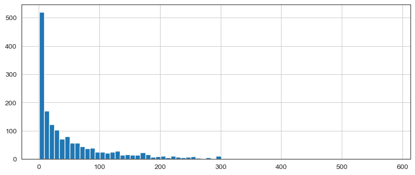
Now a few histograms:

plt.figure(figsize=(10,4))
ratings['num of ratings'].hist(bins=70)

<Axes: >

alt text

plt.figure(figsize=(10,4))
ratings['rating'].hist(bins=70)

<Axes: >

alt text

sns.jointplot(x='rating',y='num of ratings',data=ratings,alpha=0.5)

<seaborn.axisgrid.JointGrid at 0x1ee1e9d3760>

alt text

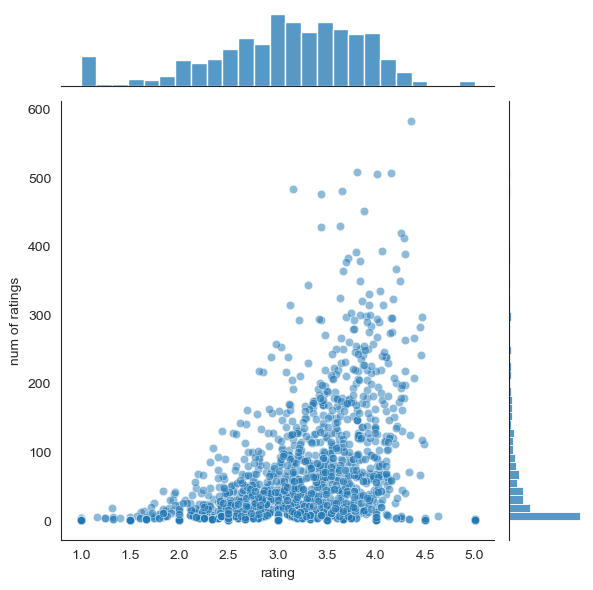
Okay! Now that we have a general idea of what the data looks like, let’s move on to creating a simple recommendation system:

Recommending Similar Movies

Now let’s create a matrix that has the user ids on one access and the movie title on another axis. Each cell will then consist of the rating the user gave to that movie. Note there will be a lot of NaN values, because most people have not seen most of the movies.

moviemat = df.pivot_table(index='user_id',columns='title',values='rating')
moviemat.head()

title	'Til There Was You (1997)	1-900 (1994)	101 Dalmatians (1996)	12 Angry Men (1957)	187 (1997)	2 Days in the Valley (1996)	20,000 Leagues Under the Sea (1954)	2001: A Space Odyssey (1968)	3 Ninjas: High Noon At Mega Mountain (1998)	39 Steps, The (1935)	...	Yankee Zulu (1994)	Year of the Horse (1997)	You So Crazy (1994)	Young Frankenstein (1974)	Young Guns (1988)	Young Guns II (1990)	Young Poisoner's Handbook, The (1995)	Zeus and Roxanne (1997)	unknown	Á köldum klaka (Cold Fever) (1994)
user_id
0	NaN	NaN	NaN	NaN	NaN	NaN	NaN	NaN	NaN	NaN	...	NaN	NaN	NaN	NaN	NaN	NaN	NaN	NaN	NaN	NaN
1	NaN	NaN	2.0	5.0	NaN	NaN	3.0	4.0	NaN	NaN	...	NaN	NaN	NaN	5.0	3.0	NaN	NaN	NaN	4.0	NaN
2	NaN	NaN	NaN	NaN	NaN	NaN	NaN	NaN	1.0	NaN	...	NaN	NaN	NaN	NaN	NaN	NaN	NaN	NaN	NaN	NaN
3	NaN	NaN	NaN	NaN	2.0	NaN	NaN	NaN	NaN	NaN	...	NaN	NaN	NaN	NaN	NaN	NaN	NaN	NaN	NaN	NaN
4	NaN	NaN	NaN	NaN	NaN	NaN	NaN	NaN	NaN	NaN	...	NaN	NaN	NaN	NaN	NaN	NaN	NaN	NaN	NaN	NaN

5 rows × 1664 columns

Most rated movie:

ratings.sort_values('num of ratings',ascending=False).head(10)

	rating	num of ratings
title
Star Wars (1977)	4.359589	584
Contact (1997)	3.803536	509
Fargo (1996)	4.155512	508
Return of the Jedi (1983)	4.007890	507
Liar Liar (1997)	3.156701	485
English Patient, The (1996)	3.656965	481
Scream (1996)	3.441423	478
Toy Story (1995)	3.878319	452
Air Force One (1997)	3.631090	431
Independence Day (ID4) (1996)	3.438228	429

Let’s choose two movies: starwars, a sci-fi movie. And Fargo, a comedy.

ratings.head()

	rating	num of ratings
title
'Til There Was You (1997)	2.333333	9
1-900 (1994)	2.600000	5
101 Dalmatians (1996)	2.908257	109
12 Angry Men (1957)	4.344000	125
187 (1997)	3.024390	41

Now let’s grab the user ratings for those two movies:

starwars_user_ratings = moviemat['Star Wars (1977)']
Fargo_user_ratings = moviemat['Fargo (1996)']
starwars_user_ratings.head()

user_id
  5.0
  5.0
  5.0
  NaN
  5.0
Name: Star Wars (1977), dtype: float64

similar_to_starwars = moviemat.corrwith(starwars_user_ratings)
similar_to_Fargo = moviemat.corrwith(Fargo_user_ratings)

We can then use corrwith() method to get correlations between two pandas series:

Let’s clean this by removing NaN values and using a DataFrame instead of a series:

corr_starwars = pd.DataFrame(similar_to_starwars,columns=['Correlation'])
corr_starwars.dropna(inplace=True)
corr_starwars.head()

	Correlation
title
'Til There Was You (1997)	0.872872
1-900 (1994)	-0.645497
101 Dalmatians (1996)	0.211132
12 Angry Men (1957)	0.184289
187 (1997)	0.027398

Now if we sort the dataframe by correlation, we should get the most similar movies, however note that we get some results that don’t really make sense. This is because there are a lot of movies only watched once by users who also watched star wars (it was the most popular movie).

corr_starwars.sort_values('Correlation',ascending=False).head(10)

	Correlation
title
Commandments (1997)	1.0
Cosi (1996)	1.0
No Escape (1994)	1.0
Stripes (1981)	1.0
Man of the Year (1995)	1.0
Hollow Reed (1996)	1.0
Beans of Egypt, Maine, The (1994)	1.0
Good Man in Africa, A (1994)	1.0
Old Lady Who Walked in the Sea, The (Vieille qui marchait dans la mer, La) (1991)	1.0
Outlaw, The (1943)	1.0

Let’s fix this by filtering out movies that have less than 100 reviews (this value was chosen based off the histogram from earlier).

corr_starwars = corr_starwars.merge(ratings,on='title', how='inner')
corr_starwars.head()

	Correlation	rating	num of ratings
title
'Til There Was You (1997)	0.872872	2.333333	9
1-900 (1994)	-0.645497	2.600000	5
101 Dalmatians (1996)	0.211132	2.908257	109
12 Angry Men (1957)	0.184289	4.344000	125
187 (1997)	0.027398	3.024390	41

Alternative Method

# corr_starwars = corr_starwars.join(ratings['num of ratings'])
# corr_starwars.head()

Now sort the values and notice how the titles make a lot more sense:

corr_starwars[corr_starwars['num of ratings']>100].sort_values('Correlation',ascending=False).head()

	Correlation	rating	num of ratings
title
Star Wars (1977)	1.000000	4.359589	584
Empire Strikes Back, The (1980)	0.748353	4.206522	368
Return of the Jedi (1983)	0.672556	4.007890	507
Raiders of the Lost Ark (1981)	0.536117	4.252381	420
Austin Powers: International Man of Mystery (1997)	0.377433	3.246154	130

Now the same for the Fargo:

corr_Fargo = pd.DataFrame(similar_to_Fargo,columns=['Correlation'])
corr_Fargo.dropna(inplace=True)
corr_Fargo = corr_Fargo.join(ratings['num of ratings'])
corr_Fargo[corr_Fargo['num of ratings']>100].sort_values('Correlation',ascending=False).head()

	Correlation	num of ratings
title
Fargo (1996)	1.000000	508
Sling Blade (1996)	0.381159	136
Lone Star (1996)	0.370915	187
Quiz Show (1994)	0.355031	175
Lawrence of Arabia (1962)	0.353408	173

Arezoo Khalili

Data Science Portfolio

Movie Recommendation System- Finding Similar Movies

Import Libraries

Get the Data

EDA

Visualization Imports

Recommending Similar Movies

Alternative Method