University Classification- Applying KMeans Clustering to Distinguish Between Private and Public Institutions
For this project, I will attempt to employ KMeans Clustering cluster Universities into two groups of Private and Public, using the data that I have.
KMeans clustering is an unsupervised learning algorithm. In this project, although the data includes labels (Private or Public), the labels were used only for evaluation purposes after clustering. KMeans itself does not use these labels during its clustering process, making it suitable for exploring patterns and structures within the data without prior classification information.
Project Overview
Context
I would like to create a model that allows me to use a few features of universities to cluster them into two groups of Private and Public. Information about the universities is in the dataset ‘College_Data’. The College dataset has 777 rows and 18 columns named as:
- Private: A factor with levels No and Yes indicating private or public university
- Apps: Number of applications received
- Accept: Number of applications accepted
- Enroll: Number of new students enrolled
- Top10perc Pct.: new students from top 10% of H.S. class
- Top25perc Pct.: new students from top 25% of H.S. class
- F. Undergrad: Number of fulltime undergraduates
- P.Undergrad: Number of parttime undergraduates
- Outstate: Out-of-state tuition
- Room.Board: Room and board costs
- Books: Estimated book costs
- Personal: Estimated personal spending
- PhD: Pct. of faculty with Ph.D.’s
- Terminal: Pct. of faculty with terminal degree
- S.F.Ratio: Student/faculty ratio
- perc.alumni: Pct. alumni who donate
- Expend: Instructional expenditure per student
- Grad.Rate: Graduation rate
Importing Required Packages
import pandas as pd
import numpy as np
import matplotlib.pyplot as plt
import seaborn as sns
from sklearn.cluster import KMeans
from sklearn.metrics import confusion_matrix,classification_report
Getting the Data
df = pd.read_csv('College_Data',index_col=0)
Checking the dataset
df.head()
| Private | Apps | Accept | Enroll | Top10perc | Top25perc | F.Undergrad | P.Undergrad | Outstate | Room.Board | Books | Personal | PhD | Terminal | S.F.Ratio | perc.alumni | Expend | Grad.Rate | |
|---|---|---|---|---|---|---|---|---|---|---|---|---|---|---|---|---|---|---|
| Abilene Christian University | Yes | 1660 | 1232 | 721 | 23 | 52 | 2885 | 537 | 7440 | 3300 | 450 | 2200 | 70 | 78 | 18.1 | 12 | 7041 | 60 |
| Adelphi University | Yes | 2186 | 1924 | 512 | 16 | 29 | 2683 | 1227 | 12280 | 6450 | 750 | 1500 | 29 | 30 | 12.2 | 16 | 10527 | 56 |
| Adrian College | Yes | 1428 | 1097 | 336 | 22 | 50 | 1036 | 99 | 11250 | 3750 | 400 | 1165 | 53 | 66 | 12.9 | 30 | 8735 | 54 |
| Agnes Scott College | Yes | 417 | 349 | 137 | 60 | 89 | 510 | 63 | 12960 | 5450 | 450 | 875 | 92 | 97 | 7.7 | 37 | 19016 | 59 |
| Alaska Pacific University | Yes | 193 | 146 | 55 | 16 | 44 | 249 | 869 | 7560 | 4120 | 800 | 1500 | 76 | 72 | 11.9 | 2 | 10922 | 15 |
df.info()
<class 'pandas.core.frame.DataFrame'>
Index: 777 entries, Abilene Christian University to York College of Pennsylvania
Data columns (total 18 columns):
 #   Column       Non-Null Count  Dtype
---  ------       --------------  -----
 0   Private      777 non-null    object
 1   Apps         777 non-null    int64
 2   Accept       777 non-null    int64
 3   Enroll       777 non-null    int64
 4   Top10perc    777 non-null    int64
 5   Top25perc    777 non-null    int64
 6   F.Undergrad  777 non-null    int64
 7   P.Undergrad  777 non-null    int64
 8   Outstate     777 non-null    int64
 9   Room.Board   777 non-null    int64
 10  Books        777 non-null    int64
 11  Personal     777 non-null    int64
 12  PhD          777 non-null    int64
 13  Terminal     777 non-null    int64
 14  S.F.Ratio    777 non-null    float64
 15  perc.alumni  777 non-null    int64
 16  Expend       777 non-null    int64
 17  Grad.Rate    777 non-null    int64
dtypes: float64(1), int64(16), object(1)
memory usage: 115.3+ KB
df.describe()
| Apps | Accept | Enroll | Top10perc | Top25perc | F.Undergrad | P.Undergrad | Outstate | Room.Board | Books | Personal | PhD | Terminal | S.F.Ratio | perc.alumni | Expend | Grad.Rate | |
|---|---|---|---|---|---|---|---|---|---|---|---|---|---|---|---|---|---|
| count | 777.000000 | 777.000000 | 777.000000 | 777.000000 | 777.000000 | 777.000000 | 777.000000 | 777.000000 | 777.000000 | 777.000000 | 777.000000 | 777.000000 | 777.000000 | 777.000000 | 777.000000 | 777.000000 | 777.00000 |
| mean | 3001.638353 | 2018.804376 | 779.972973 | 27.558559 | 55.796654 | 3699.907336 | 855.298584 | 10440.669241 | 4357.526384 | 549.380952 | 1340.642214 | 72.660232 | 79.702703 | 14.089704 | 22.743887 | 9660.171171 | 65.46332 |
| std | 3870.201484 | 2451.113971 | 929.176190 | 17.640364 | 19.804778 | 4850.420531 | 1522.431887 | 4023.016484 | 1096.696416 | 165.105360 | 677.071454 | 16.328155 | 14.722359 | 3.958349 | 12.391801 | 5221.768440 | 17.17771 |
| min | 81.000000 | 72.000000 | 35.000000 | 1.000000 | 9.000000 | 139.000000 | 1.000000 | 2340.000000 | 1780.000000 | 96.000000 | 250.000000 | 8.000000 | 24.000000 | 2.500000 | 0.000000 | 3186.000000 | 10.00000 |
| 25% | 776.000000 | 604.000000 | 242.000000 | 15.000000 | 41.000000 | 992.000000 | 95.000000 | 7320.000000 | 3597.000000 | 470.000000 | 850.000000 | 62.000000 | 71.000000 | 11.500000 | 13.000000 | 6751.000000 | 53.00000 |
| 50% | 1558.000000 | 1110.000000 | 434.000000 | 23.000000 | 54.000000 | 1707.000000 | 353.000000 | 9990.000000 | 4200.000000 | 500.000000 | 1200.000000 | 75.000000 | 82.000000 | 13.600000 | 21.000000 | 8377.000000 | 65.00000 |
| 75% | 3624.000000 | 2424.000000 | 902.000000 | 35.000000 | 69.000000 | 4005.000000 | 967.000000 | 12925.000000 | 5050.000000 | 600.000000 | 1700.000000 | 85.000000 | 92.000000 | 16.500000 | 31.000000 | 10830.000000 | 78.00000 |
| max | 48094.000000 | 26330.000000 | 6392.000000 | 96.000000 | 100.000000 | 31643.000000 | 21836.000000 | 21700.000000 | 8124.000000 | 2340.000000 | 6800.000000 | 103.000000 | 100.000000 | 39.800000 | 64.000000 | 56233.000000 | 118.00000 |
Exploratory Data Analysis (EDA)
It’s time to create some data visualizations!
Creating a scatterplot of Grad.Rate versus Room.Board where the points are colored by the Private column.
sns.set_style('whitegrid')
sns.lmplot(x='Room.Board',y='Grad.Rate',data=df, hue='Private',
           palette='coolwarm',height=6,aspect=1,fit_reg=False)
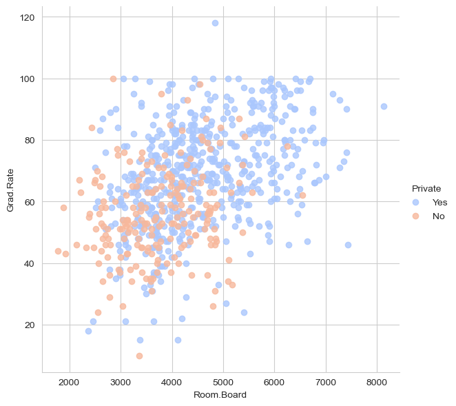
There is a clear correlation between increasing room and board costs (room.board) and higher graduation rates (Grad.Rate).
Creating a scatterplot of F.Undergrad versus Outstate where the points are colored by the Private column
sns.set_style('whitegrid')
sns.lmplot(x='Outstate',y='F.Undergrad',data=df, hue='Private',
           palette='coolwarm',height=6,aspect=1,fit_reg=False)
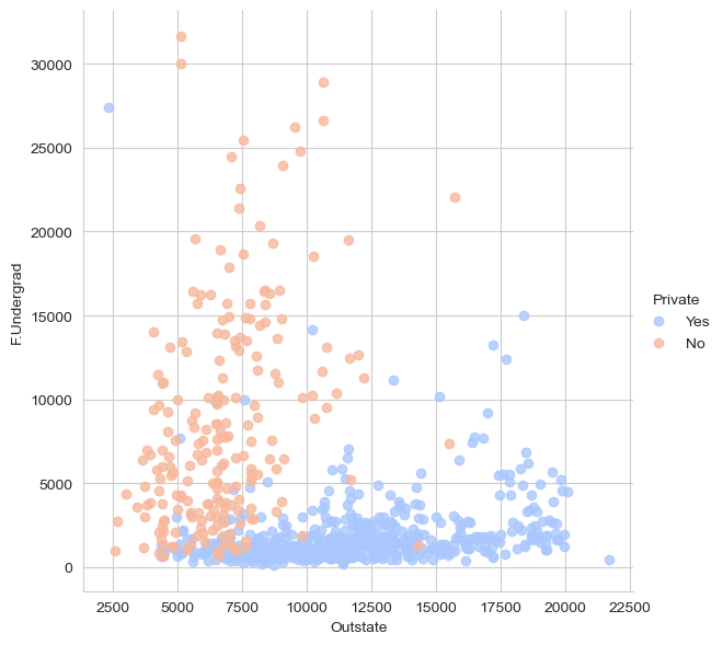
As Outstate (out-of-state tuition) increases, there is a noticeable decrease in the F.Undergrad (number of full-time students) attending private universities.
Finding if there is a school with a graduation rate of higher than 100%. What is the name of that school?
df[df['Grad.Rate']>100]
| Private | Apps | Accept | Enroll | Top10perc | Top25perc | F.Undergrad | P.Undergrad | Outstate | Room.Board | Books | Personal | PhD | Terminal | S.F.Ratio | perc.alumni | Expend | Grad.Rate | |
|---|---|---|---|---|---|---|---|---|---|---|---|---|---|---|---|---|---|---|
| Cazenovia College | Yes | 3847 | 3433 | 527 | 9 | 35 | 1010 | 12 | 9384 | 4840 | 600 | 500 | 22 | 47 | 14.3 | 20 | 7697 | 118 |
** Setting that school’s graduation rate to 100 so it makes sense.
df['Grad.Rate']['Cazenovia College'] = 100
df.loc['Cazenovia College']
Private         Yes
Apps           3847
Accept         3433
Enroll          527
Top10perc         9
Top25perc        35
F.Undergrad    1010
P.Undergrad      12
Outstate       9384
Room.Board     4840
Books           600
Personal        500
PhD              22
Terminal         47
S.F.Ratio      14.3
perc.alumni      20
Expend         7697
Grad.Rate       100
Name: Cazenovia College, dtype: object
df[df['Grad.Rate']>100]
| Private | Apps | Accept | Enroll | Top10perc | Top25perc | F.Undergrad | P.Undergrad | Outstate | Room.Board | Books | Personal | PhD | Terminal | S.F.Ratio | perc.alumni | Expend | Grad.Rate |
|---|
K Means Cluster Creation
Now it is time to create the Cluster labels!
Creating an instance of a K Means model with 2 clusters
kmeans = KMeans(n_clusters=2)
Creating input variable
X = df.drop('Private', axis = 1)
Fitting the model to all the data except for the Private label
kmeans.fit(X)
Finding the cluster center vectors
kmeans.cluster_centers_
array([[1.81323468e+03, 1.28716592e+03, 4.91044843e+02, 2.53094170e+01,
        5.34708520e+01, 2.18854858e+03, 5.95458894e+02, 1.03957085e+04,
        4.31136472e+03, 5.41982063e+02, 1.28033632e+03, 7.04424514e+01,
        7.78251121e+01, 1.40997010e+01, 2.31748879e+01, 8.93204634e+03,
        6.50926756e+01],
       [1.03631389e+04, 6.55089815e+03, 2.56972222e+03, 4.14907407e+01,
        7.02037037e+01, 1.30619352e+04, 2.46486111e+03, 1.07191759e+04,
        4.64347222e+03, 5.95212963e+02, 1.71420370e+03, 8.63981481e+01,
        9.13333333e+01, 1.40277778e+01, 2.00740741e+01, 1.41705000e+04,
        6.75925926e+01]])
Evaluation
There is no perfect way to evaluate clustering if you don’t have the labels, however since this is just an exercise, we do have the labels, so I take advantage of this to evaluate my clusters. I compared the clusters generated by KMeans with the actual labels (private vs. public) present in the dataset. This supervised evaluation indicated that the clustering algorithm largely captured the underlying structure of the data, aligning closely with the known classifications.
Creating a new column for df called ‘Cluster’, which is a 1 for a Private school, and a 0 for a public school
def converter(cluster):
    if cluster=='Yes':
        return 1
    else:
        return 0
df['Cluster'] = df['Private'].apply(converter)
df.head()
| Private | Apps | Accept | Enroll | Top10perc | Top25perc | F.Undergrad | P.Undergrad | Outstate | Room.Board | Books | Personal | PhD | Terminal | S.F.Ratio | perc.alumni | Expend | Grad.Rate | Cluster | |
|---|---|---|---|---|---|---|---|---|---|---|---|---|---|---|---|---|---|---|---|
| Abilene Christian University | Yes | 1660 | 1232 | 721 | 23 | 52 | 2885 | 537 | 7440 | 3300 | 450 | 2200 | 70 | 78 | 18.1 | 12 | 7041 | 60 | 1 |
| Adelphi University | Yes | 2186 | 1924 | 512 | 16 | 29 | 2683 | 1227 | 12280 | 6450 | 750 | 1500 | 29 | 30 | 12.2 | 16 | 10527 | 56 | 1 |
| Adrian College | Yes | 1428 | 1097 | 336 | 22 | 50 | 1036 | 99 | 11250 | 3750 | 400 | 1165 | 53 | 66 | 12.9 | 30 | 8735 | 54 | 1 |
| Agnes Scott College | Yes | 417 | 349 | 137 | 60 | 89 | 510 | 63 | 12960 | 5450 | 450 | 875 | 92 | 97 | 7.7 | 37 | 19016 | 59 | 1 |
| Alaska Pacific University | Yes | 193 | 146 | 55 | 16 | 44 | 249 | 869 | 7560 | 4120 | 800 | 1500 | 76 | 72 | 11.9 | 2 | 10922 | 15 | 1 |
Creating a confusion matrix and classification report to see how well the Kmeans clustering worked without being given any labels
print(confusion_matrix(df['Cluster'],kmeans.labels_))
print(classification_report(df['Cluster'],kmeans.labels_))
[[138  74]
 [531  34]]
              precision    recall  f1-score   support

           0       0.21      0.65      0.31       212
           1       0.31      0.06      0.10       565

    accuracy                           0.22       777
   macro avg       0.26      0.36      0.21       777
weighted avg       0.29      0.22      0.16       777
Not so bad considering the algorithm is purely using the features to cluster the universities into 2 distinct groups!
By leveraging machine learning algorithms, we can gain valuable insights into educational institutions that can inform policy-making, marketing strategies, and more in the realm of higher education.