Predictive Modeling for LendingClub- Investing in Borrowers' Repayment Probability
For this project, we will be exploring publicly available data from LendingClub.com. Lending Club connects people who need money (borrowers) with people who have money (investors). An investor would want to invest in people who showed a profile of having a high probability of paying you back. We will try to create a model that will help predict this.
Lending club had a very interesting year in 2016, so let’s check out some of their data and keep the context in mind. This data is from before they even went public.
We will use lending data from 2007-2010 and try to classify and predict whether or not the borrower paid back their loan in full.
Here are what the columns represent:
- credit.policy: 1 if the customer meets the credit underwriting criteria of LendingClub.com, and 0 otherwise.
- purpose: The purpose of the loan (takes values “credit_card”, “debt_consolidation”, “educational”, “major_purchase”, “small_business”, and “all_other”).
- int.rate: The interest rate of the loan, as a proportion (a rate of 11% would be stored as 0.11). Borrowers judged by LendingClub.com to be more risky are assigned higher interest rates.
- installment: The monthly installments owed by the borrower if the loan is funded.
- log.annual.inc: The natural log of the self-reported annual income of the borrower.
- dti: The debt-to-income ratio of the borrower (amount of debt divided by annual income).
- fico: The FICO credit score of the borrower.
- days.with.cr.line: The number of days the borrower has had a credit line.
- revol.bal: The borrower’s revolving balance (amount unpaid at the end of the credit card billing cycle).
- revol.util: The borrower’s revolving line utilization rate (the amount of the credit line used relative to total credit available).
- inq.last.6mths: The borrower’s number of inquiries by creditors in the last 6 months.
- delinq.2yrs: The number of times the borrower had been 30+ days past due on a payment in the past 2 years.
- pub.rec: The borrower’s number of derogatory public records (bankruptcy filings, tax liens, or judgments).
Import Required Packages
import pandas as pd
import numpy as np
import matplotlib.pyplot as plt
import seaborn as sns
%matplotlib inline
Getting the Data
loans = pd.read_csv('loan_data.csv')
** Checkking out the info(), head(), and describe() methods on loans.**
loans.info()
<class 'pandas.core.frame.DataFrame'>
RangeIndex: 9578 entries, 0 to 9577
Data columns (total 14 columns):
 #   Column             Non-Null Count  Dtype
---  ------             --------------  -----
 0   credit.policy      9578 non-null   int64
 1   purpose            9578 non-null   object
 2   int.rate           9578 non-null   float64
 3   installment        9578 non-null   float64
 4   log.annual.inc     9578 non-null   float64
 5   dti                9578 non-null   float64
 6   fico               9578 non-null   int64
 7   days.with.cr.line  9578 non-null   float64
 8   revol.bal          9578 non-null   int64
 9   revol.util         9578 non-null   float64
 10  inq.last.6mths     9578 non-null   int64
 11  delinq.2yrs        9578 non-null   int64
 12  pub.rec            9578 non-null   int64
 13  not.fully.paid     9578 non-null   int64
dtypes: float64(6), int64(7), object(1)
memory usage: 1.0+ MB
loans.describe()
| credit.policy | int.rate | installment | log.annual.inc | dti | fico | days.with.cr.line | revol.bal | revol.util | inq.last.6mths | delinq.2yrs | pub.rec | not.fully.paid | |
|---|---|---|---|---|---|---|---|---|---|---|---|---|---|
| count | 9578.000000 | 9578.000000 | 9578.000000 | 9578.000000 | 9578.000000 | 9578.000000 | 9578.000000 | 9.578000e+03 | 9578.000000 | 9578.000000 | 9578.000000 | 9578.000000 | 9578.000000 |
| mean | 0.804970 | 0.122640 | 319.089413 | 10.932117 | 12.606679 | 710.846314 | 4560.767197 | 1.691396e+04 | 46.799236 | 1.577469 | 0.163708 | 0.062122 | 0.160054 |
| std | 0.396245 | 0.026847 | 207.071301 | 0.614813 | 6.883970 | 37.970537 | 2496.930377 | 3.375619e+04 | 29.014417 | 2.200245 | 0.546215 | 0.262126 | 0.366676 |
| min | 0.000000 | 0.060000 | 15.670000 | 7.547502 | 0.000000 | 612.000000 | 178.958333 | 0.000000e+00 | 0.000000 | 0.000000 | 0.000000 | 0.000000 | 0.000000 |
| 25% | 1.000000 | 0.103900 | 163.770000 | 10.558414 | 7.212500 | 682.000000 | 2820.000000 | 3.187000e+03 | 22.600000 | 0.000000 | 0.000000 | 0.000000 | 0.000000 |
| 50% | 1.000000 | 0.122100 | 268.950000 | 10.928884 | 12.665000 | 707.000000 | 4139.958333 | 8.596000e+03 | 46.300000 | 1.000000 | 0.000000 | 0.000000 | 0.000000 |
| 75% | 1.000000 | 0.140700 | 432.762500 | 11.291293 | 17.950000 | 737.000000 | 5730.000000 | 1.824950e+04 | 70.900000 | 2.000000 | 0.000000 | 0.000000 | 0.000000 |
| max | 1.000000 | 0.216400 | 940.140000 | 14.528354 | 29.960000 | 827.000000 | 17639.958330 | 1.207359e+06 | 119.000000 | 33.000000 | 13.000000 | 5.000000 | 1.000000 |
loans.head()
| credit.policy | purpose | int.rate | installment | log.annual.inc | dti | fico | days.with.cr.line | revol.bal | revol.util | inq.last.6mths | delinq.2yrs | pub.rec | not.fully.paid | |
|---|---|---|---|---|---|---|---|---|---|---|---|---|---|---|
| 0 | 1 | debt_consolidation | 0.1189 | 829.10 | 11.350407 | 19.48 | 737 | 5639.958333 | 28854 | 52.1 | 0 | 0 | 0 | 0 |
| 1 | 1 | credit_card | 0.1071 | 228.22 | 11.082143 | 14.29 | 707 | 2760.000000 | 33623 | 76.7 | 0 | 0 | 0 | 0 |
| 2 | 1 | debt_consolidation | 0.1357 | 366.86 | 10.373491 | 11.63 | 682 | 4710.000000 | 3511 | 25.6 | 1 | 0 | 0 | 0 |
| 3 | 1 | debt_consolidation | 0.1008 | 162.34 | 11.350407 | 8.10 | 712 | 2699.958333 | 33667 | 73.2 | 1 | 0 | 0 | 0 |
| 4 | 1 | credit_card | 0.1426 | 102.92 | 11.299732 | 14.97 | 667 | 4066.000000 | 4740 | 39.5 | 0 | 1 | 0 | 0 |
Exploratory Data Analysis
Let’s do some data visualization! We’ll use seaborn and pandas built-in plotting capabilities.
** Creating a histogram of two FICO distributions on top of each other, one for each credit.policy outcome.**
plt.figure(figsize=(10,6))

loans[loans['credit.policy']==1]['fico'].hist(alpha=0.5, color='green',
                                              bins=30,label='Credit.Policy=1')
loans[loans['credit.policy']==0]['fico'].hist(alpha=0.5,color='red',
                                              bins=30,label='Credit.Policy=0')
plt.legend()
plt.xlabel('FICO')
Text(0.5, 0, 'FICO')
We can see more people in the data set have credit policy of 1 than 0. Also, people with lower fisco have credit policy of 0.
** Creating a similar figure, except this time select by the not.fully.paid column.**
plt.figure(figsize=(10,6))

loans[loans['not.fully.paid']==0]['fico'].hist(alpha=0.5,color='yellow',
                                              bins=30,label='not.fully.paid=0')
loans[loans['not.fully.paid']==1]['fico'].hist(alpha=0.5, color='blue',
                                              bins=30,label='not.fully.paid=1')
plt.legend()
plt.xlabel('FICO')
Text(0.5, 0, 'FICO')
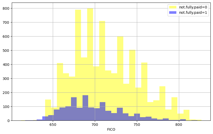
A similar trend can be seen for both not fully paid =0 and =1. Some spikes are also visible at certain points that might be attributed to the fico policy
** Creating a countplot using seaborn showing the counts of loans by purpose, with the color hue defined by not.fully.paid. **
plt.figure(figsize=(11,7))

sns.countplot(loans, x= 'purpose', hue = 'not.fully.paid')
<Axes: xlabel='purpose', ylabel='count'>
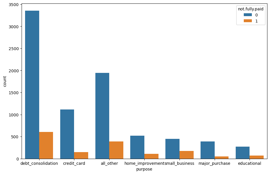
Debt seems to be the most popular reason for getting loan abd credit card and home improvement come next.
sns.jointplot(loans, x='fico', y='int.rate')
<seaborn.axisgrid.JointGrid at 0x21a907c93f0>
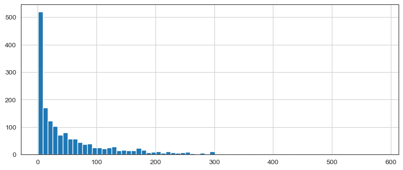
As fico score increases, we will have better credit score and you are paying lower ineterest rates
Setting up the Data for our Random Forest Classification Model!
Check loans.info() again.
loans.info()
<class 'pandas.core.frame.DataFrame'>
RangeIndex: 9578 entries, 0 to 9577
Data columns (total 14 columns):
 #   Column             Non-Null Count  Dtype
---  ------             --------------  -----
 0   credit.policy      9578 non-null   int64
 1   purpose            9578 non-null   object
 2   int.rate           9578 non-null   float64
 3   installment        9578 non-null   float64
 4   log.annual.inc     9578 non-null   float64
 5   dti                9578 non-null   float64
 6   fico               9578 non-null   int64
 7   days.with.cr.line  9578 non-null   float64
 8   revol.bal          9578 non-null   int64
 9   revol.util         9578 non-null   float64
 10  inq.last.6mths     9578 non-null   int64
 11  delinq.2yrs        9578 non-null   int64
 12  pub.rec            9578 non-null   int64
 13  not.fully.paid     9578 non-null   int64
dtypes: float64(6), int64(7), object(1)
memory usage: 1.0+ MB
Categorical Features
The purpose column is categorical
Therefore, we need to transform them using OneHotEncoder.
Let’s show you a way of dealing with these columns that can be expanded to multiple categorical features if necessary.
Create a list of 1 element containing the string ‘purpose’. Call this list cat_feats.
from sklearn.preprocessing import OneHotEncoder

# Create a list of categorical variables
categorical_vars = ['purpose']

# Create and apply OneHotEncoder while removing the dummy variable
one_hot_encoder = OneHotEncoder(sparse = False, drop = 'first')

# Apply fit_transform on training data
loans_encoded = one_hot_encoder.fit_transform(loans[categorical_vars])

# Get feature names to see what each column in the 'encoder_vars_array' presents
encoder_feature_names = one_hot_encoder.get_feature_names_out(categorical_vars)

# Convert our result from an array to a DataFrame
loans_encoded = pd.DataFrame(loans_encoded, columns = encoder_feature_names)

# Concatenate (Link together in a series or chain) new DataFrame to our original DataFrame
loans = pd.concat([loans.reset_index(drop = True),loans_encoded.reset_index(drop = True)], axis = 1)

# Drop the original categorical variable columns
loans.drop(categorical_vars, axis = 1, inplace = True)
C:\Users\arezo\anaconda3\lib\site-packages\sklearn\preprocessing\_encoders.py:828: FutureWarning: `sparse` was renamed to `sparse_output` in version 1.2 and will be removed in 1.4. `sparse_output` is ignored unless you leave `sparse` to its default value.
  warnings.warn(
loans.info()
<class 'pandas.core.frame.DataFrame'>
RangeIndex: 9578 entries, 0 to 9577
Data columns (total 19 columns):
 #   Column                      Non-Null Count  Dtype
---  ------                      --------------  -----
 0   credit.policy               9578 non-null   int64
 1   int.rate                    9578 non-null   float64
 2   installment                 9578 non-null   float64
 3   log.annual.inc              9578 non-null   float64
 4   dti                         9578 non-null   float64
 5   fico                        9578 non-null   int64
 6   days.with.cr.line           9578 non-null   float64
 7   revol.bal                   9578 non-null   int64
 8   revol.util                  9578 non-null   float64
 9   inq.last.6mths              9578 non-null   int64
 10  delinq.2yrs                 9578 non-null   int64
 11  pub.rec                     9578 non-null   int64
 12  not.fully.paid              9578 non-null   int64
 13  purpose_credit_card         9578 non-null   float64
 14  purpose_debt_consolidation  9578 non-null   float64
 15  purpose_educational         9578 non-null   float64
 16  purpose_home_improvement    9578 non-null   float64
 17  purpose_major_purchase      9578 non-null   float64
 18  purpose_small_business      9578 non-null   float64
dtypes: float64(12), int64(7)
memory usage: 1.4 MB
Train Test Split
Now it’s time to split our data into a training set and a testing set!
from sklearn.model_selection import train_test_split
X = loans.drop('not.fully.paid',axis=1)
y = loans['not.fully.paid']
X_train, X_test, y_train, y_test = train_test_split(X, y, test_size=0.20, random_state=42)
Training a Decision Tree Model
Let’s start by training a single decision tree first!
** Importing DecisionTreeClassifier**
from sklearn.tree import DecisionTreeClassifier
Creating an instance of DecisionTreeClassifier() called dtree and fit it to the training data.
dtree = DecisionTreeClassifier()
dtree.fit(X_train,y_train)
DecisionTreeClassifier()In a Jupyter environment, please rerun this cell to show the HTML representation or trust the notebook.
On GitHub, the HTML representation is unable to render, please try loading this page with nbviewer.org.
DecisionTreeClassifier()
Predictions and Evaluation of Decision Tree
Creating predictions from the test set and creating a classification report and a confusion matrix.
y_predict = dtree.predict(X_test)
from sklearn.metrics import classification_report,confusion_matrix
print(classification_report(y_test,y_predict))
              precision    recall  f1-score   support

           0       0.85      0.83      0.84      1611
           1       0.20      0.23      0.22       305

    accuracy                           0.73      1916
   macro avg       0.53      0.53      0.53      1916
weighted avg       0.75      0.73      0.74      1916
print(confusion_matrix(y_test,y_predict))
[[1336  275]
 [ 235   70]]
Training the Random Forest model
Now it’s time to train our model!
Creating an instance of the RandomForestClassifier class and fitting it to our training data from the previous step.
from sklearn.ensemble import RandomForestClassifier
rfc = RandomForestClassifier(n_estimators=600)
rfc.fit(X_train,y_train)
RandomForestClassifier(n_estimators=600)In a Jupyter environment, please rerun this cell to show the HTML representation or trust the notebook.
On GitHub, the HTML representation is unable to render, please try loading this page with nbviewer.org.
RandomForestClassifier(n_estimators=600)
Predictions and Evaluation
Let’s predict the y_test values and evaluate our model.
** Predicting the class of not.fully.paid for the X_test data.**
y_predict = rfc.predict(X_test)
Now creating a classification report from the results.
from sklearn.metrics import classification_report,confusion_matrix
print(classification_report(y_test,y_predict))
              precision    recall  f1-score   support

           0       0.84      0.99      0.91      1611
           1       0.31      0.01      0.03       305

    accuracy                           0.84      1916
   macro avg       0.57      0.50      0.47      1916
weighted avg       0.76      0.84      0.77      1916
Showing the Confusion Matrix for the predictions.
print(confusion_matrix(y_test,y_predict))
[[1602    9]
 [ 301    4]]