In the rapidly evolving financial services industry, companies strive to provide accurate and personalized offerings to their clients. An insurance agency working with a leading financial services provider, embarked on a mission to enhance their life insurance offerings by leveraging the power of machine learning. This initiative aimed to design a platform that would give clients access to predict premiums for a combined life insurance and investment package with greater accuracy, ensuring fair pricing and personalized plans.
Project Overview
Context
The agency serves a broad spectrum of clients, each with unique financial needs and health profiles. Traditionally, calculating life insurance premiums involved a complex evaluation of multiple factors, often leading to discrepancies and inefficiencies. While financial advisors have access to software for evaluating different plans and determining premiums, the agency wants to empower clients with a platform that allows them to get a rough estimate of their premiums based on their specific budget and status, as well as the potential savings.
Actions
To tackle this challenge, a comprehensive data-driven approach was adopted. The journey began with the collection of extensive client data, including demographic information, health metrics, and lifestyle factors. This data was then meticulously preprocessed to ensure its accuracy and completeness.
I built a predictive model to find relationships between client metrics and life insurance premium for previous clients, and used this to predict premiums for potential new clients.
As I was predicting a numeric output, I tested three regression modeling approaches, namely:
- Linear Regression
- Decision Tree
- Random Forest
Results
The Random Forest had the highest predictive accuracy.
Metric 1: R-Squared (Test Set)
- Random Forest = 0.917
- Decision Tree = 0.908
- Linear Regression = 0.766
Metric 2: Cross Validated R-Squared (K-Fold Cross Validation, k = 4)
- Random Forest = 0.883
- Decision Tree = 0.865
- Linear Regression = 0.756
As the most important outcome for this project was predictive accuracy, rather than explicitly understanding weighted drivers of prediction, I chose the Random Forest as the model to use for making predictions on the life insurance premiums for future clients.
Key Definition
age: client’s age
sex: client’s gender
bmi: Body mass index is a value derived from the mass and height of a person (the body mass (kg) divided by the square of the body height (m^2))
children: number of client’s children
smoker: client’s smoking status
region: client’s place of residence
CI: includes critical illness insurance
rated: increased premium due to health problems
UL permanent: combined investment and life insurance
disability: includes disability insurance
premium: client’s monthly payment
Data Overview
The initial dataset included various attributes such as age, gender, BMI, number of children, smoking status, region, and several insurance-related features. To prepare the data for modeling, several key steps were undertaken:
Handling Missing Values: Any missing values in the dataset were identified and appropriately addressed.
Dealing with Outliers: The dataset was examined for outliers to ensure the integrity of the data.
Encoding Categorical Variables: Categorical variables like gender, smoker status, and region were encoded using one-hot encoding to make them suitable for machine learning models.
Feature Scaling: Numerical features were standardized to ensure they were on a comparable scale, enhancing the model’s performance.
Model Training and Evaluation
With the data prepared, the next step was to train a machine learning model capable of accurately predicting life insurance premiums.
I tested three regression modeling approaches, namely:
- Linear Regression
- Decision Tree
- Random Forest
For each model, I imported the data in the same way but needed to pre-process the data based on the requirements of each particular algorithm. I trained & tested each model, refined each to provide optimal performance, and then measured this predictive performance based on several metrics to give a well-rounded overview of which is best.
The dataset was split into training and testing sets, ensuring that the model could be evaluated on unseen data. The model was trained on the training set, and its performance was evaluated using the testing set. Key metric of R-squared was calculated to assess the model’s accuracy.
To further refine the model, cross-validation was performed using KFold, providing a more robust evaluation by splitting the data into multiple folds and ensuring the model’s consistency across different subsets of the data.
Linear Regression
I utilized the scikit-learn library within Python to model the data using Linear Regression.
# Import Required Packages

import pandas as pd
import matplotlib.pyplot as plt
import seaborn as sns

from sklearn.model_selection import train_test_split, cross_val_score, KFold
from sklearn.linear_model import LinearRegression
from sklearn.utils import shuffle
from sklearn.preprocessing import OneHotEncoder
from sklearn.metrics import r2_score

# Import Sample Data

data_for_model = pd.read_excel('Life insurance.xlsx', sheet_name='Life insurance')

# Shuffle data
data_for_model = shuffle(data_for_model, random_state = 42)

# Get Data Information

data_for_model.info()
data_for_model['region'].value_counts()

# Deal with Missing Values

data_for_model.isna().sum()
Outliers
The ability of a Linear Regression model to generalize well across all data could be hampered if there were outliers present. There was no right or wrong way to deal with outliers, but it was always something worth very careful consideration - just because a value was high or low, did not necessarily mean it should not be there! In this code section, I used .describe() from Pandas to investigate the spread of values for each of the predictors.
# Deal with Outliers

outlier_investigation = data_for_model.describe()
The results of this can be seen in the table below.
| Metric | Age | BMI | Children | Premium |
|---|---|---|---|---|
| Count | 1338 | 1338 | 1338 | 1338 |
| Mean | 39.2 | 30.67 | 1.09 | 1104.10 |
| Std | 14.05 | 6.10 | 1.21 | 1010.11 |
| Min | 18 | 16 | 0 | 93.49 |
| 25% | 27 | 26.3 | 0 | 391.28 |
| 50% | 39 | 30.4 | 1 | 775.27 |
| 75% | 51 | 34.7 | 2 | 1386.66 |
| Max | 64 | 53.1 | 5 | 5314.20 |
Based on this investigation, I saw some max column values for bmi was much higher than the median value.
Because of this, I applied some outlier removal to facilitate generalization across the full dataset.
I did this using the “boxplot approach” where I removed any rows where the values within those columns were outside of the interquartile range multiplied by 2.
outlier_columns = ["bmi"]

# boxplot approach
for column in outlier_columns:

    lower_quartile = data_for_model[column].quantile(0.25)
    upper_quartile = data_for_model[column].quantile(0.75)
    iqr = upper_quartile - lower_quartile
    iqr_extended = iqr * 2
    min_border = lower_quartile - iqr_extended
    max_border = upper_quartile + iqr_extended

    outliers = data_for_model[(data_for_model[column] < min_border) | (data_for_model[column] > max_border)].index
    print(f"{len(outliers)} outliers detected in column {column}")

    data_for_model.drop(outliers, inplace = True)
Split Out Data For Modelling
# Split Input Variables and Output Variables

X = data_for_model.drop(['premium'], axis = 1)
y = data_for_model['premium']

# Split out Training and Test Sets

X_train, X_test, y_train, y_test = train_test_split (X, y, test_size = 0.2, random_state = 42)
Categorical Predictor Variables
In my dataset, I had seven categorical variables. As the Linear Regression algorithm could only deal with numerical data, I had to encode my categorical variables.
One Hot Encoding was used to represent categorical variables as binary vectors.
For ease, after I applied One Hot Encoding, I turned my training and test objects back into Pandas Dataframes, with the column names applied.
# Deal with Categorical Variables

# Create a list of categorical variables
categorical_vars = ['sex', 'smoker', 'region', 'CI', 'rated', 'UL permanent', 'disability']

# Create and apply OneHotEncoder while removing the dummy variable
one_hot_encoder = OneHotEncoder(sparse = False, drop = 'first')

# Apply fit_transform on training data
X_train_encoded =  one_hot_encoder.fit_transform(X_train[categorical_vars])

# Apply transform on test data
X_test_encoded = one_hot_encoder.transform(X_test[categorical_vars])

# Get feature names to see what each column in the 'encoder_vars_array' presents
encoder_feature_names = one_hot_encoder.get_feature_names_out(categorical_vars)

# Convert our result from an array to a DataFrame
X_train_encoded = pd.DataFrame(X_train_encoded, columns = encoder_feature_names)
X_test_encoded = pd.DataFrame(X_test_encoded, columns = encoder_feature_names)

# Concatenate (Link together in a series or chain) new DataFrame to our original DataFrame
X_train = pd.concat([X_train.reset_index(drop = True), X_train_encoded.reset_index(drop = True)], axis = 1)
X_test = pd.concat([X_test.reset_index(drop = True), X_test_encoded.reset_index(drop = True)], axis = 1)

# Drop the original categorical variable columns
X_train.drop(categorical_vars, axis = 1, inplace = True)
X_test.drop(categorical_vars, axis = 1, inplace = True)
Data Visualization
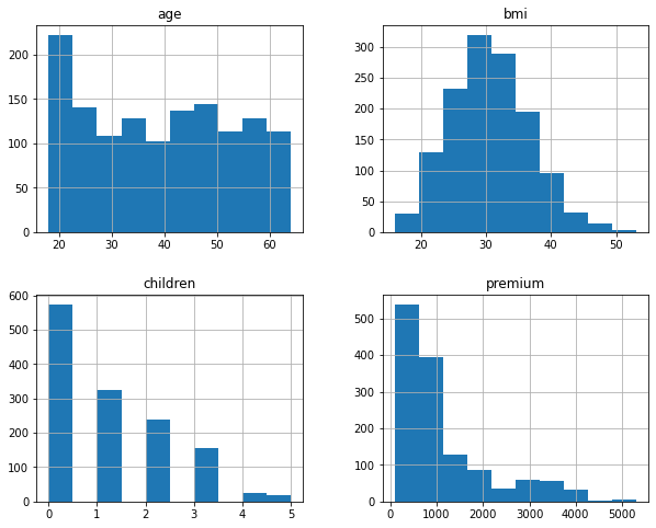
# Data Distribution
data_for_model.hist(figsize=(10,8))
This created the below plot, which showed where the majority of data points lied.
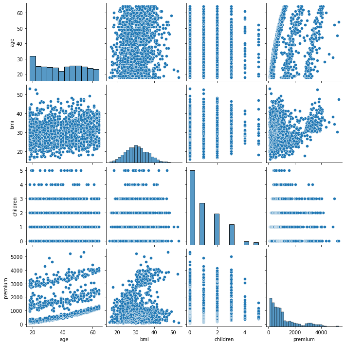
# Pairplot
sns.pairplot(data_for_model)
Following pairplot showed the correlation between bmi and age with premium.
-
A positive correlation between bmi and premium suggests that clients with higher BMI might have higher premiums. This could be due to the increased health risks associated with higher bmi.
-
A positive correlation between age and premium indicates that older clients tend to have higher premiums. This is expected as life insurance premiums generally increase with age due to higher risk.
Feature selection and feature scaling did not impact the modeling process or the accuracy of the predictions. Therefore, they were excluded.
Model Training
Instantiating and training the Linear Regression model was done using the below code:
# instantiate my model object
regressor = LinearRegression()

# fit my model using our training & test sets
regressor.fit(X_train, y_train)
Model Performance Assessment
Predict On The Test Set
To assess how well my model was predicting new data - I used the trained model object (here called regressor) and asked it to predict the insurance premium variable for the test set.
# predict on the test set
y_pred = regressor.predict(X_test)
Calculate R-Squared
R-Squared is a metric that shows the percentage of variance in the output variable y that is being explained by the input variable(s) x. It is a value that ranges between 0 and 1, with a higher value showing a higher level of explained variance.
r_squared = r2_score(y_test, y_pred)
print(r_squared)
The resulting R-squared score from this was 0.766.
Calculate Cross Validated R-Squared (Cross validation (KFold: including both shuffling and the random state))
An even more powerful and reliable way to assess model performance is to utilize Cross Validation.
Instead of simply dividing our data into a single training set, and a single test set, with Cross Validation we can break our data into several “chunks” and then iteratively train the model on all but one of the “chunks”, test the model on the remaining “chunk” until each has had a chance to be the test set.
The result of this is that we are provided a number of test set validation results - and we can take the average of these to give a much more robust & reliable view of how our model will perform on new, unseen data!
In the code below, I put this into place. I first specified that I wanted 4 “chunks” and then I passed in my regressor object, training set, and test set. I also specified the metric I wanted to assess with, in this case, I sticked to R-squared.
Finally, I took a mean of all four test set results.
cv = KFold(n_splits = 4, shuffle = True, random_state = 42)
cv_scores = cross_val_score(regressor, X_train, y_train, cv = cv, scoring = 'r2')     # returns r2 for each chunk of data (each cv)
cv_scores.mean()
print(cv_scores.mean())
The resulting R-squared score from this was 0.755 which as expected, was slightly lower than the score I got for R-squared on it’s own.
Model Summary Statistics
Although my overall goal for this project was predictive accuracy, rather than an explicit understanding of the relationships of each of the input variables and the output variable, it was always interesting to look at the summary statistics for these.
The coefficient value for each of the input variables, along with that of the intercept would make up the equation for the line of best fit for this particular model (or more accurately, in this case, it would be the plane of best fit, as I had multiple input variables).
# Extract model coefficients
coefficients = pd.DataFrame(regressor.coef_)
input_variable_names = pd.DataFrame(X_train.columns)
summary_stats = pd.concat([input_variable_names, coefficients], axis = 1)
summary_stats.columns = ['input_variable', 'coefficient']

# Extract model intercept
regressor.intercept_
Decision Tree
I again utilized the scikit-learn library within Python to model my data using a Decision Tree. The whole code can be found below:
# Import Required Packages
import pandas as pd
import matplotlib.pyplot as plt
import seaborn as sns

from sklearn.model_selection import train_test_split, cross_val_score, KFold
from sklearn.utils import shuffle
from sklearn.preprocessing import OneHotEncoder
from sklearn.metrics import r2_score
from sklearn.tree import DecisionTreeRegressor, plot_tree

# Import Sample Data
data_for_model = pd.read_excel('Life insurance.xlsx', sheet_name='Life insurance')

# Shuffle data
data_for_model = shuffle(data_for_model, random_state = 42)

# Get Data Information
data_for_model.info()
data_for_model['region'].value_counts()
While Linear Regression is susceptible to the effects of outliers, and highly correlated input variables - Decision Trees are not, so the required preprocessing here was lighter. I still however put in place logic for:
Missing Values
# Deal with Missing Values
data_for_model.isna().sum()
There was no missing values in the data.
Split Out Data For Modelling
# Split Input Variables and Output Variables
X = data_for_model.drop(['premium'], axis = 1)
y = data_for_model['premium']

# Split out Training and Test Sets
X_train, X_test, y_train, y_test = train_test_split (X, y, test_size = 0.2, random_state = 42)
Categorical Predictor Variables
We would again apply One Hot Encoding to the categorical column.
# Create a list of categorical variables
categorical_vars = ['sex', 'smoker', 'region', 'CI', 'rated', 'UL permanent', 'disability']

# Create and apply OneHotEncoder while removing the dummy variable
one_hot_encoder = OneHotEncoder(sparse = False, drop = 'first')

# Apply fit_transform on training data
X_train_encoded =  one_hot_encoder.fit_transform(X_train[categorical_vars])

# Apply transform on test data
X_test_encoded = one_hot_encoder.transform(X_test[categorical_vars])

# Get feature names to see what each column in the 'encoder_vars_array' presents
encoder_feature_names = one_hot_encoder.get_feature_names_out(categorical_vars)

# Convert our result from an array to a DataFrame
X_train_encoded = pd.DataFrame(X_train_encoded, columns = encoder_feature_names)
X_test_encoded = pd.DataFrame(X_test_encoded, columns = encoder_feature_names)

# Concatenate (Link together in a series or chain) new DataFrame to our original DataFrame
X_train = pd.concat([X_train.reset_index(drop = True), X_train_encoded.reset_index(drop = True)], axis = 1)
X_test = pd.concat([X_test.reset_index(drop = True), X_test_encoded.reset_index(drop = True)], axis = 1)

# Drop the original categorical variable columns
X_train.drop(categorical_vars, axis = 1, inplace = True)
X_test.drop(categorical_vars, axis = 1, inplace = True)
Model Training
Instantiating and training the Decision Tree model was done using the below code. I used the random_state parameter to ensure I got reproducible results, and this helped us understand any improvements in performance with changes to model hyperparameters.
# Model Training
regressor = DecisionTreeRegressor(random_state = 42, max_depth = 4)
regressor.fit(X_train, y_train)
Model Performance Assessment
# Predict on the test set
y_pred = regressor.predict(X_test)

# Model Assessment (Validation)

# First approach: Calculate R-squared
r_squared = r2_score(y_test, y_pred)
print(r_squared)

# Calculate Cross Validated R-Squared (Cross validation (KFold: including both shuffling and the random state))
cv = KFold(n_splits = 4, shuffle = True, random_state = 42)                    # n_splits: number of equally sized chunk of data
cv_scores = cross_val_score(regressor, X_train, y_train, cv = cv, scoring = 'r2')
cv_scores.mean()
print(cv_scores.mean())
The resulting R-squared and cross-validated R-squared scores from this analysis was 0.908 and 0.865, respectively.
Decision Tree Regularisation
Decision Trees can be prone to over-fitting, in other words, without any limits on their splitting, they will end up learning the training data perfectly. We would much prefer our model to have a more generalized set of rules, as this will be more robust & reliable when making predictions on new data.
One effective method of avoiding this over-fitting is to apply a max depth to the Decision Tree, meaning we only allow it to split the data a certain number of times before it is required to stop.
Unfortunately, we don’t necessarily know the best number of splits to use for this - so below I looped over a variety of values and assessed which gave me the best predictive performance!
Finding the best max depth
max_depth_list = list(range(1,9))
accuracy_scores = []
for depth in max_depth_list:
regressor = DecisionTreeRegressor(max_depth = depth, random_state = 42)
regressor.fit(X_train, y_train)
y_pred = regressor.predict(X_test)
accuracy = r2_score(y_test,y_pred)
accuracy_scores.append(accuracy)
max_accuracy = max(accuracy_scores)
max_accuracy_idx = accuracy_scores.index(max_accuracy)
optimal_depth = max_depth_list[max_accuracy_idx]
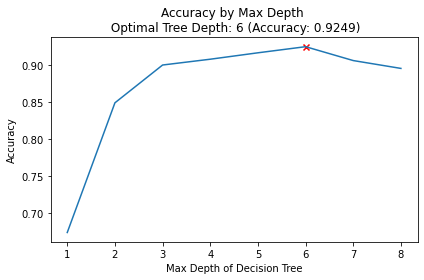
# Plot of max depths
plt.plot(max_depth_list, accuracy_scores)
plt.scatter(optimal_depth, max_accuracy, marker = 'x', color = 'red')
plt.title(f'Accuracy by Max Depth \n Optimal Tree Depth: {optimal_depth} (Accuracy: {round(max_accuracy, 4)})')
plt.xlabel('Max Depth of Decision Tree')
plt.ylabel('Accuracy')
plt.tight_layout()
plt.show()
Best max depth was 6 but refitting the model with max depth of 6 did not change the validation score.
Random Forest
I utilized the scikit-learn library within Python to model my data using a Random Forest.
# Import required packages
import pandas as pd
import matplotlib.pyplot as plt
import seaborn as sns

from sklearn.model_selection import train_test_split, cross_val_score, KFold
from sklearn.utils import shuffle
from sklearn.preprocessing import OneHotEncoder
from sklearn.metrics import r2_score
from sklearn.ensemble import RandomForestRegressor
from sklearn.inspection import permutation_importance

# Import Sample Data
data_for_model = pd.read_excel('Life insurance.xlsx', sheet_name='Life insurance')

# Shuffle data
data_for_model = shuffle(data_for_model, random_state = 42)

# Get Data Information
data_for_model.info()
data_for_model['region'].value_counts()

# Deal with Missing Values
data_for_model.isna().sum()
Split Out Data For Modelling
# Split Input Variables and Output Variables
X = data_for_model.drop(['premium'], axis = 1)
y = data_for_model['premium']

# Split out Training and Test Sets
X_train, X_test, y_train, y_test = train_test_split (X, y, test_size = 0.2, random_state = 42)
Categorical Predictor Variables
# Create a list of categorical variables
categorical_vars = ['sex', 'smoker', 'region', 'CI', 'rated', 'UL permanent', 'disability']

# Create and apply OneHotEncoder while removing the dummy variable
one_hot_encoder = OneHotEncoder(sparse = False, drop = 'first')

# Apply fit_transform on training data
X_train_encoded =  one_hot_encoder.fit_transform(X_train[categorical_vars])

# Apply transform on test data
X_test_encoded = one_hot_encoder.transform(X_test[categorical_vars])

# Get feature names to see what each column in the 'encoder_vars_array' presents
encoder_feature_names = one_hot_encoder.get_feature_names_out(categorical_vars)

# Convert our result from an array to a DataFrame
X_train_encoded = pd.DataFrame(X_train_encoded, columns = encoder_feature_names)
X_test_encoded = pd.DataFrame(X_test_encoded, columns = encoder_feature_names)

# Concatenate (Link together in a series or chain) new DataFrame to our original DataFrame
X_train = pd.concat([X_train.reset_index(drop = True), X_train_encoded.reset_index(drop = True)], axis = 1)
X_test = pd.concat([X_test.reset_index(drop = True), X_test_encoded.reset_index(drop = True)], axis = 1)

# Drop the original categorical variable columns
X_train.drop(categorical_vars, axis = 1, inplace = True)
X_test.drop(categorical_vars, axis = 1, inplace = True)
Model Training
# instantiate my model object
regressor = RandomForestRegressor(random_state = 42)

# fit my model using my training & test sets
regressor.fit(X_train, y_train)
Model Performance Assessment
Predict On The Test Set
# predict on the test set
y_pred = regressor.predict(X_test)
Calculate R-Squared
# calculate r-squared for our test set predictions
r_squared = r2_score(y_test, y_pred)
print(r_squared)
The resulting r-squared score from this was 0.917 - higher than both Linear Regression & the Decision Tree.
Calculate Cross Validated R-Squared
As I did when testing Linear Regression & Decision Tree, I again utilized Cross Validation.
# calculate the mean cross-validated r-squared for the test set predictions
cv = KFold(n_splits = 4, shuffle = True, random_state = 42)
cv_scores = cross_val_score(regressor, X_train, y_train, cv = cv, scoring = "r2")
cv_scores.mean()
The mean cross-validated r-squared score from this was 0.883 which again was higher than what I saw for both Linear Regression & Decision Tree.
Feature Importance
Random Forests are an ensemble model, made up of many, many Decision Trees, each of which was different due to the randomness of the data being provided, and the random selection of input variables available at each potential split point.
Because of this, I ended up with a powerful and robust model, but because of the random or different nature of all these Decision trees - the model gave me a unique insight into how important each of my input variables was to the overall model.
At a high level, in a Random Forest, I could measure importance by asking How much would accuracy decrease if a specific input variable was removed or randomized?
If this decrease in performance, or accuracy, was large, then I’d deem that input variable to be quite important, and if I saw only a small decrease in accuracy, then I’d conclude that the variable is of less importance.
At a high level, there were two common ways to tackle this. The first, often just called Feature Importance is where we find all nodes in the Decision Trees of the forest where a particular input variable is used to split the data and assess what the Mean Squared Error (for a Regression problem) was before the split was made, and compare this to the Mean Squared Error after the split was made. We can take the average of these improvements across all Decision Trees in the Random Forest to get a score that tells us how much better we’re making the model by using that input variable.
If we do this for each of my input variables, we can compare these scores and understand which is adding the most value to the predictive power of the model!
The other approach, often called Permutation Importance cleverly uses some data that has gone unused at when random samples are selected for each Decision Tree (this stage is called “bootstrap sampling” or “bootstrapping”)
These observations that were not randomly selected for each Decision Tree are known as Out of Bag observations and these can be used for testing the accuracy of each particular Decision Tree.
For each Decision Tree, all of the Out of Bag observations are gathered and then passed through. Once all of these observations have been run through the Decision Tree, we obtain an accuracy score for these predictions, which in the case of a regression problem could be Mean Squared Error or r-squared.
In order to understand the importance, we randomize the values within one of the input variables - a process that essentially destroys any relationship that might exist between that input variable and the output variable - and run that updated data through the Decision Tree again, obtaining a second accuracy score. The difference between the original accuracy and the new accuracy gives us a view on how important that particular variable is for predicting the output.
Permutation Importance is often preferred over Feature Importance which can at times inflate the importance of numerical features. Both are useful and in most cases will give fairly similar results.
Here, I put them both in place and plotted the results…
# calculate feature importance
feature_importance = pd.DataFrame(regressor.feature_importances_)
feature_names = pd.DataFrame(X_train.columns)
feature_importance_summary = pd.concat([feature_names, feature_importance], axis = 1)
feature_importance_summary.columns = ['input_variable', 'feature_importance']
feature_importance_summary.sort_values(by = 'feature_importance', inplace = True)

plt.barh(feature_importance_summary['input_variable'], feature_importance_summary['feature_importance'])
plt.title('Feature Importance of Random Forest')
plt.xlabel('Feature Importance')
plt.tight_layout()
plt.show()

# calculate permutation importance
result = permutation_importance(regressor, X_test, y_test, n_repeats = 10, random_state = 42)      # n_repeats: How many times we want to apply random shuffling on each input variable

permutation_importance = pd.DataFrame(result['importances_mean'])                                  # importances_mean: average of data we got over n_repeats of random shuffling
permutation_names = pd.DataFrame(X_train.columns)
permutation_importance_summary = pd.concat([feature_names, permutation_importance], axis = 1)
permutation_importance_summary.columns = ['input_variable', 'permutation_importance']
permutation_importance_summary.sort_values(by = 'permutation_importance', inplace = True)

plt.barh(permutation_importance_summary['input_variable'],permutation_importance_summary['permutation_importance'])
plt.title('Permutation Importance of Random Forest')
plt.xlabel('Permutation Importance')
plt.tight_layout()
plt.show()
That code gave me the below plots - the first being for Feature Importance and the second for Permutation Importance!
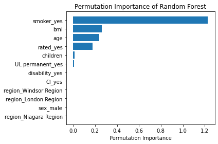
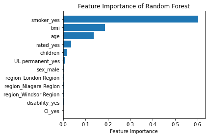
The overall story from both approaches was very similar, in that by far, the most important or impactful input variable was smoking status, followed by bmi and age. These insights were consistent with the results from my assessments using Linear Regression and Decision Tree models.
Growth & Next Steps
Impact and Future Directions:
By accurately predicting life insurance premiums, the agency can offer fairer and more personalized insurance plans to their clients, enhancing customer satisfaction and trust. It would also allow clients to play with premiums and see how different premiums could allocate money for their retirements.
Looking ahead, the insurance agency plans to continuously refine and expand this model by incorporating additional data sources and exploring more advanced machine learning techniques. This initiative represents a commitment to innovation and excellence, paving the way for a more efficient and customer-centric future.