Obesity Level Classification Using Eating Habits and Physical Condition
🧠 Project Overview
This project leverages supervised machine learning to classify individuals into obesity categories based on their demographic data, eating habits, and physical activity levels. The dataset consists of 2,111 observations and 17 features, capturing both behavioral and physiological variables.
The target variable, NObeyesdad, represents seven distinct obesity classes:
- Insufficient Weight
- Normal Weight
- Overweight Level I
- Overweight Level II
- Obesity Type I
- Obesity Type II
- Obesity Type III
Dataset Source: UCI Machine Learning Repository
📊 Dataset Summary
- 📌 Rows: 2,111
- 📌 Features: 16 predictors + 1 target (
NObeyesdad) - 📌 Balance: 77% synthetic (via SMOTE), 23% survey-based real data
- 📌 Goal: Predict obesity level using lifestyle and physiological variables
📁 Feature Categories
- 🥗 Eating Habits:
- FAVC (Frequent consumption of high-calorie food)
- FCVC (Frequency of vegetable consumption)
- NCP (Number of daily meals)
- CAEC (Food consumption between meals)
- CH2O (Daily water intake)
- CALC (Alcohol consumption)
- 🏃♂️ Physical Activity & Lifestyle:
- FAF (Physical activity frequency)
- SCC (Calorie consumption monitoring)
- TUE (Technology usage per day)
- MTRANS (Transportation mode)
- 👤 Demographics:
- Gender
- Age
- Height
- Weight
- Family_History_with_Overweight
- 🎯 Target Variable:
NObeyesdad(Multi-class label indicating obesity category)
Each row in the dataset corresponds to one individual, capturing their nutritional behavior, lifestyle factors, and physical condition. These features provide a comprehensive view of potential predictors for obesity and are used to train classification models.
📦 Import Required Packages and Dataset
%load_ext dotenv
%dotenv
The dotenv extension is already loaded. To reload it, use:
%reload_ext dotenv
# Import standard libraries
import pandas as pd
import matplotlib.pyplot as plt
import seaborn as sns
import warnings
warnings.filterwarnings('ignore')
import os
import sys

# **Append source directory to Python path**
sys.path.append(os.getenv('SRC_DIR'))
📥 Load the Dataset into a DataFrame
# Load the dataset
from DataManager import get_data

obesity_df = get_data('../data/ObesityDataSet_raw_and_data_sinthetic.csv')
obesity_df.shape
Output: (2111, 17)
🔍 Display Basic Information
obesity_df.head()
| Gender | Age | Height | Weight | family_history_with_overweight | FAVC | FCVC | NCP | CAEC | SMOKE | CH2O | SCC | FAF | TUE | CALC | MTRANS | NObeyesdad | |
|---|---|---|---|---|---|---|---|---|---|---|---|---|---|---|---|---|---|
| 0 | Female | 21.0 | 1.62 | 64.0 | yes | no | 2.0 | 3.0 | Sometimes | no | 2.0 | no | 0.0 | 1.0 | no | Public_Transportation | Normal_Weight |
| 1 | Female | 21.0 | 1.52 | 56.0 | yes | no | 3.0 | 3.0 | Sometimes | yes | 3.0 | yes | 3.0 | 0.0 | Sometimes | Public_Transportation | Normal_Weight |
| 2 | Male | 23.0 | 1.80 | 77.0 | yes | no | 2.0 | 3.0 | Sometimes | no | 2.0 | no | 2.0 | 1.0 | Frequently | Public_Transportation | Normal_Weight |
| 3 | Male | 27.0 | 1.80 | 87.0 | no | no | 3.0 | 3.0 | Sometimes | no | 2.0 | no | 2.0 | 0.0 | Frequently | Walking | Overweight_Level_I |
| 4 | Male | 22.0 | 1.78 | 89.8 | no | no | 2.0 | 1.0 | Sometimes | no | 2.0 | no | 0.0 | 0.0 | Sometimes | Public_Transportation | Overweight_Level_II |
📝 Rename Columns for Clarity
# Rename columns for improved readability
columnName = {'family_history_with_overweight': 'Family_History',
                                          'FAVC' : 'High_Cal_Foods_Frequently',
                                          'FCVC': 'Freq_Veg', 'NCP': 'Num_Meals',
                                          'CAEC': 'Snacking',
                                          'SMOKE': 'Smoke',
                                          'CH2O': 'Water_Intake',
                                          'SCC': 'Calorie_Monitoring' ,
                                          'FAF': 'Phys_Activity',
                                          'TUE': 'Tech_Use', 'CALC':
                                          "Freq_Alcohol",
                                          'MTRANS': 'Transportation',
                                          'NObeyesdad': 'Obesity_Level'}


obesity_df_renamed = obesity_df.rename(columns=columnName)
ℹ️ Dataset Info After Renaming
obesity_df_renamed.info()
<class 'pandas.core.frame.DataFrame'>
RangeIndex: 2111 entries, 0 to 2110
Data columns (total 17 columns):
 #   Column                     Non-Null Count  Dtype
---  ------                     --------------  -----
 0   Gender                     2111 non-null   object
 1   Age                        2111 non-null   float64
 2   Height                     2111 non-null   float64
 3   Weight                     2111 non-null   float64
 4   Family_History             2111 non-null   object
 5   High_Cal_Foods_Frequently  2111 non-null   object
 6   Freq_Veg                   2111 non-null   float64
 7   Num_Meals                  2111 non-null   float64
 8   Snacking                   2111 non-null   object
 9   Smoke                      2111 non-null   object
 10  Water_Intake               2111 non-null   float64
 11  Calorie_Monitoring         2111 non-null   object
 12  Phys_Activity              2111 non-null   float64
 13  Tech_Use                   2111 non-null   float64
 14  Freq_Alcohol               2111 non-null   object
 15  Transportation             2111 non-null   object
 16  Obesity_Level              2111 non-null   object
dtypes: float64(8), object(9)
memory usage: 280.5+ KB
📊 Summary Statistics
obesity_df_renamed.describe()
| Age | Height | Weight | Freq_Veg | Num_Meals | Water_Intake | Phys_Activity | Tech_Use | |
|---|---|---|---|---|---|---|---|---|
| count | 2111.000000 | 2111.000000 | 2111.000000 | 2111.000000 | 2111.000000 | 2111.000000 | 2111.000000 | 2111.000000 |
| mean | 24.312600 | 1.701677 | 86.586058 | 2.419043 | 2.685628 | 2.008011 | 1.010298 | 0.657866 |
| std | 6.345968 | 0.093305 | 26.191172 | 0.533927 | 0.778039 | 0.612953 | 0.850592 | 0.608927 |
| min | 14.000000 | 1.450000 | 39.000000 | 1.000000 | 1.000000 | 1.000000 | 0.000000 | 0.000000 |
| 25% | 19.947192 | 1.630000 | 65.473343 | 2.000000 | 2.658738 | 1.584812 | 0.124505 | 0.000000 |
| 50% | 22.777890 | 1.700499 | 83.000000 | 2.385502 | 3.000000 | 2.000000 | 1.000000 | 0.625350 |
| 75% | 26.000000 | 1.768464 | 107.430682 | 3.000000 | 3.000000 | 2.477420 | 1.666678 | 1.000000 |
| max | 61.000000 | 1.980000 | 173.000000 | 3.000000 | 4.000000 | 3.000000 | 3.000000 | 2.000000 |
🧹 Data Preprocessing
In this section, we perform essential data quality checks to prepare the dataset for analysis:
-
Check for Missing or Null Values
Confirm that no values are missing from the dataset. -
Check for Uniqueness in Categories
Verify the categorical variables contain consistent and non-redundant entries. -
Check for Duplicates
Identify and remove duplicate records to ensure data integrity. -
Check for Outliers
Detect and assess the impact of outliers on numerical features using statistical and visual methods.
📌 Identify Numerical vs Categorical Columns
num_col = obesity_df_renamed.select_dtypes(include=['float64', 'int64']).columns
cat_col = obesity_df_renamed.select_dtypes(include=['object']).columns
✅ Missing or Null Values
# Find missing values
obesity_df_renamed.isna().sum()
Gender                       0
Age                          0
Height                       0
Weight                       0
Family_History               0
High_Cal_Foods_Frequently    0
Freq_Veg                     0
Num_Meals                    0
Snacking                     0
Smoke                        0
Water_Intake                 0
Calorie_Monitoring           0
Phys_Activity                0
Tech_Use                     0
Freq_Alcohol                 0
Transportation               0
Obesity_Level                0
dtype: int64
Observation:
✅ No missing or null values were found in the dataset. No imputation is required.
obesity_df_renamed.isnull().sum() # check for null values
Gender                       0
Age                          0
Height                       0
Weight                       0
Family_History               0
High_Cal_Foods_Frequently    0
Freq_Veg                     0
Num_Meals                    0
Snacking                     0
Smoke                        0
Water_Intake                 0
Calorie_Monitoring           0
Phys_Activity                0
Tech_Use                     0
Freq_Alcohol                 0
Transportation               0
Obesity_Level                0
dtype: int64
Similarly with missing values data doesn’t have any null values.
🧾 Uniqueness Check for Categorical Variables
unique_values_per_column = {col: obesity_df_renamed[col].unique() for col in cat_col}

# Display unique values for each column
for col, unique_vals in unique_values_per_column.items():
    print(f"Unique values in '{col}': {unique_vals}")
Unique values in 'Gender': ['Female' 'Male']
Unique values in 'Family_History': ['yes' 'no']
Unique values in 'High_Cal_Foods_Frequently': ['no' 'yes']
Unique values in 'Snacking': ['Sometimes' 'Frequently' 'Always' 'no']
Unique values in 'Smoke': ['no' 'yes']
Unique values in 'Calorie_Monitoring': ['no' 'yes']
Unique values in 'Freq_Alcohol': ['no' 'Sometimes' 'Frequently' 'Always']
Unique values in 'Transportation': ['Public_Transportation' 'Walking' 'Automobile' 'Motorbike' 'Bike']
Unique values in 'Obesity_Level': ['Normal_Weight' 'Overweight_Level_I' 'Overweight_Level_II'
 'Obesity_Type_I' 'Insufficient_Weight' 'Obesity_Type_II'
 'Obesity_Type_III']
Observation:
✅ All categorical variables contain consistent and interpretable values. No cleaning required.
🔁 Duplicate Rows
obesity_df_renamed.duplicated().sum()
np.int64(24)
🟡 24 duplicate rows detected
# Show duplicated values if needed

#obesity_df_renamed[obesity_df_renamed.duplicated(keep=False)]
Remove duplicates
# remove duplicates from the dataset
from DataManager import drop_duplicates

data = drop_duplicates(obesity_df_renamed)
data.shape
Observation:
✅ Duplicates removed successfully
🚨 Outlier Detection (IQR Method)
def find_outliers_IQR(df,numeric_col):

   q1=df[numeric_col].quantile(0.25)
   q3=df[numeric_col].quantile(0.75)
   IQR=q3-q1
   outliers = df[((df[numeric_col]<(q1-1.5*IQR)) | (df[numeric_col]>(q3+1.5*IQR)))]
   return outliers

numeric_columns = num_col
for column in numeric_columns:
    outliers = find_outliers_IQR(data, column)

    if outliers.empty:
        print(f"No outliers detected in column {column}")
    else:
        print(f"{len(outliers)} outliers detected in column {column}")
        print("Max outlier value:", str(outliers[column].max()))
        print("Min outlier value:", str(outliers[column].min()))
Observation:
✅ Detected outliers in:
Age: 167 values
Height: 1 value
Weight: 1 value
Num_Meals: 577 values
📦 Boxplots for Visual Outlier Analysis
We will visualize only the columns we have outliers
for column in num_col:
    outliers = find_outliers_IQR(data, column)
    if not outliers.empty:  # Only plot if outliers are present
        plt.figure(figsize=(8, 6))
        plt.boxplot(data[column].dropna(), vert=False, patch_artist=True)
        plt.title(f"Box Plot for {column} (Outliers Detected)")
        plt.xlabel(column)
        plt.grid(True)
        plt.show()
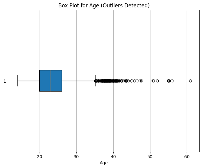
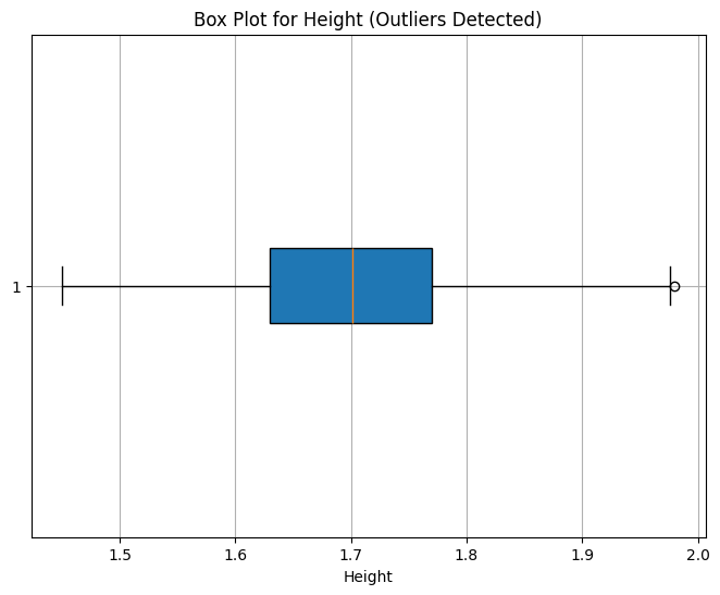
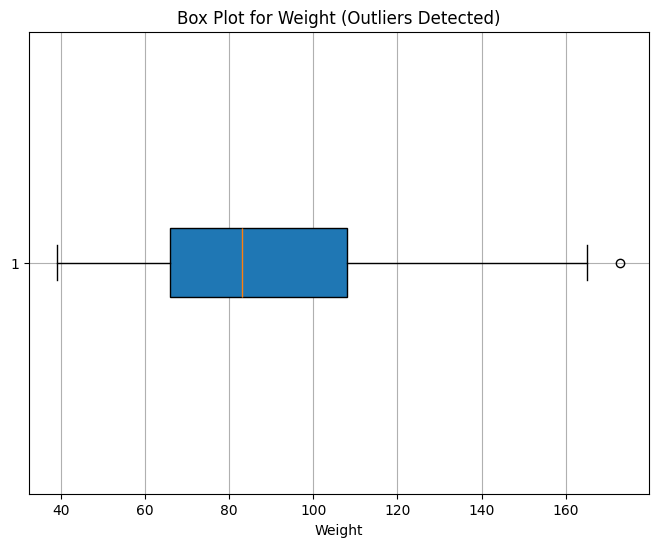
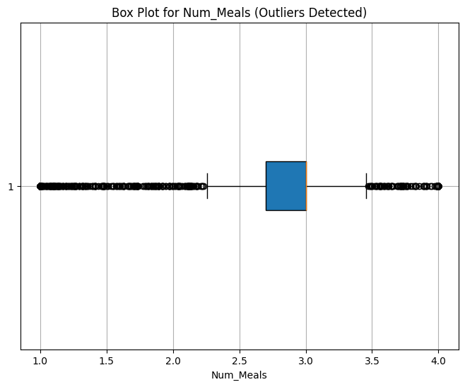
Outlier Interpretation
Age is right-skewed. We’ll retain outliers and revisit during feature engineering.
Num_Meals behaves like a categorical variable. We’ll retain all values as they may be informative.
Height and Weight outliers are minimal and reasonable, so we retain them.
📊 Distribution of Age
# Age distribution across different obesity levels (NObeyesdad)

plt.figure(figsize=(10,8))
nobeyesdad_order = ['Insufficient_Weight', 'Normal_Weight', 'Overweight_Level_I','Overweight_Level_II','Obesity_Type_I', 'Obesity_Type_II', 'Obesity_Type_III']  # Adjust according to your dataset
sns.boxplot(x='Obesity_Level', y='Age', data=data, palette='Set3', order=nobeyesdad_order)
plt.title('Age Distribution across Obesity Levels (Obesity_Level)')
plt.xlabel('Obesity Level (Obesity_Level)')
plt.ylabel('Age')
plt.xticks(rotation=45)
plt.tight_layout()
plt.show()
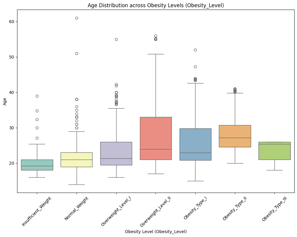
From the figure below, it is evident that Age is right-skewed, suggesting that the dataset predominantly represents certain age groups. This could introduce a bias in the machine learning decision-making process. For now, we will retain the outliers and observe how the skewness of the Age feature impacts the model’s performance. Depending on the results, we will decide whether to keep or remove the outliers during the feature engineering phase.
sns.histplot(data['Age'], kde=True, bins=20, color='skyblue')
plt.title('Age Distribution')
Text(0.5, 1.0, 'Age Distribution')
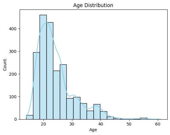
Observation:
✅ Age values range from 14 to 61. We’ll retain all entries for now.
📈 Target Class Distribution
# Define the order of obesity levels based on their frequency
nobeyesdad_order = data['Obesity_Level'].value_counts().index

plt.figure(figsize=(10,8))
sns.countplot(x='Obesity_Level', data=data, palette='Set3', order=nobeyesdad_order)
plt.title('Distribution of Obesity Levels (Obesity_Level)')
plt.xlabel('Obesity Level')
plt.ylabel('Count')
plt.xticks(rotation=45)
plt.tight_layout()
plt.show()
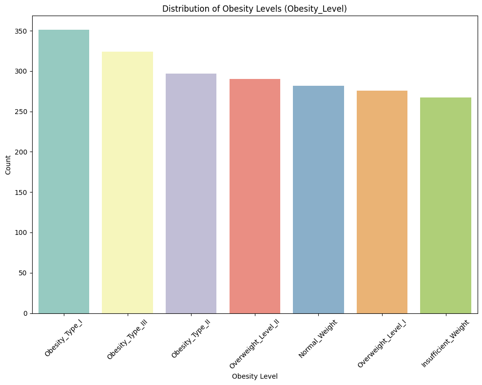
Observation:
✅ Obesity Type I is the most frequent category.
🔍 Pairplot of Numerical Features
sns.pairplot(data[['Age', 'Height', 'Weight', 'Freq_Veg', 'Water_Intake', 'Phys_Activity', 'Obesity_Level']], hue='Obesity_Level', palette='Set3')
plt.show()
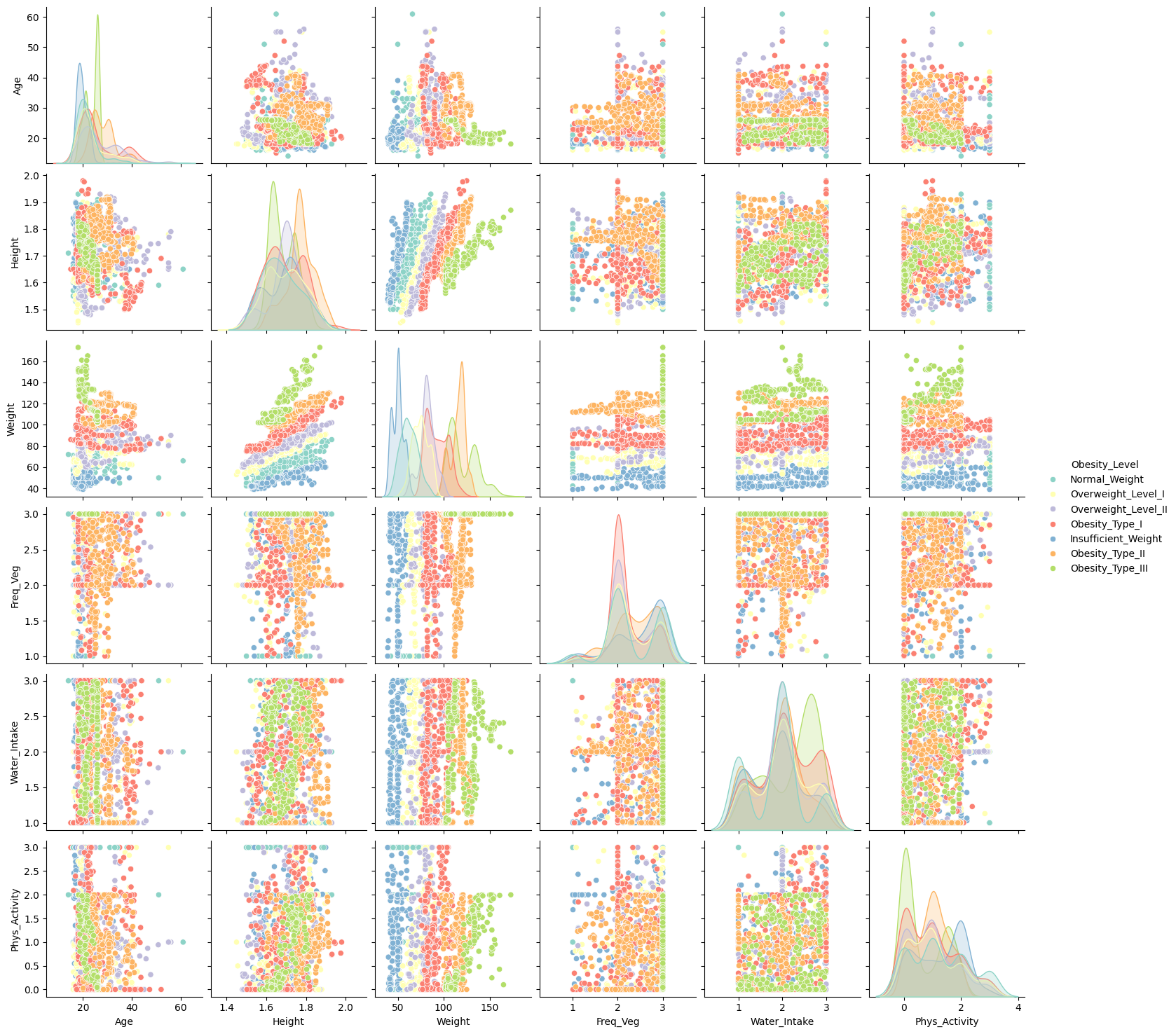
Observation:
✅ Height and Weight show strong correlation. Consider engineering BMI.
Other features, such as Frequency of Vegetable Consumption (FCVC), Water Intake (CH2O), and Physical Activity Frequency (FAF), do not exhibit a clear linear relationship with other variables. However, their monolithic behavior (clustered values) suggests they may behave more like categorical features despite being numerical. This observation should be considered in the preprocessing and modeling stages to ensure these features are treated appropriately.
📊 Categorical Feature Distribution by Target
# Plot categorical variables against Obesity_Level
binary_palette = {"yes": "#8dd3c7", "no": "#fb8072"}
# Define the desired order of obesity levels
obesity_level_order = [
    "Insufficient_Weight",
    "Normal_Weight",
    "Overweight_Level_I",
    "Overweight_Level_II",
    "Obesity_Type_I",
    "Obesity_Type_II",
    "Obesity_Type_III"
]
plt.figure(figsize=(12, 170))
counter = 1
for var in cat_col:
    if counter < len(cat_col):
        plt.subplot(20, 1, counter)
        plt.title(f"{var} vs Obesity_Level")

        # Determine the appropriate palette based on variable categories
        if var in ["Family_History", "High_Cal_Foods_Frequently", "Smoke", "Calorie_Monitoring"]:
            palette = binary_palette  # Use "yes" and "no" palette
        else:
            palette = "Set3"  # Default palette for other categorical variables

        # Plot with the selected palette
        sns.countplot(
            x="Obesity_Level",
            hue=var,
            data=obesity_df_renamed,
            edgecolor="black",
            palette=palette,
            order=obesity_level_order
        )
    counter += 1
plt.tight_layout()
plt.show()
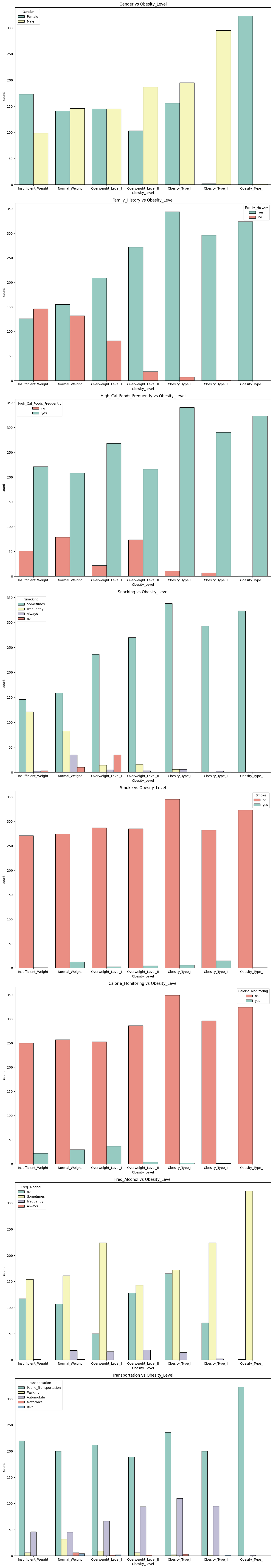
🧠 Insights from Categorical Analysis
-
Gender: Slight imbalance in Obesity II & III (more males).
-
Family_History: Clear link with higher obesity.
-
FAVC: High-calorie food consumption increases with obesity.
-
Snacking: “Sometimes” snacking is more frequent in overweight/obese groups.
-
SMOKE: No significant pattern with obesity.
-
SCC (Calorie Monitoring): Lower monitoring in higher obesity levels.
-
CALC (Alcohol): No strong pattern observed.
-
MTRANS: Walkers tend to be in lower obesity levels.
🔗 Correlation Matrix of Numerical Features
We will perform correlation analysis between numerical features with using Pearson Correlation coefficent.
# Create a heatmap for the correlation matrix using only numerical columns
numerical_columns = obesity_df_renamed.select_dtypes(include=['float64', 'int64']).columns
numerical_correlation_matrix = obesity_df_renamed[numerical_columns].corr()

# Plot the heatmap
plt.figure(figsize=(10, 8))
sns.heatmap(numerical_correlation_matrix, annot=True, cmap='coolwarm', fmt='.2f')
plt.title('Correlation Matrix of Numerical Variables')
plt.show()
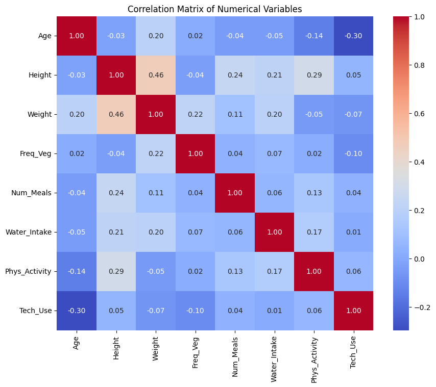
Observation:
✅ Strong positive correlation observed between Height and Weight. 💡 We will define a new feature: BMI = Weight / Height² in the next section.
📐 Feature Engineering: Body Mass Index (BMI) Calculation
We introduce a new feature BMI (Body Mass Index) to better capture the interaction between weight and height, and explore its impact on obesity classification.
# Define new BMI feature
data['BMI'] = data['Weight'] / (data['Height'] ** 2)
📊 Exploratory Analysis on BMI
📈 BMI Distribution Across Obesity Levels
plt.figure(figsize=(10,8))
nobeyesdad_order = ['Insufficient_Weight', 'Normal_Weight', 'Overweight_Level_I','Overweight_Level_II','Obesity_Type_I', 'Obesity_Type_II', 'Obesity_Type_III']  # Adjust according to your dataset
sns.boxplot(x='Obesity_Level', y='BMI', data=data, palette='Set3', order=nobeyesdad_order)
plt.title('BMI Distribution across Obesity Levels (Obesity_Level)')
plt.xlabel('Obesity Level (Obesity_Level)')
plt.ylabel('BMI')
plt.xticks(rotation=45)
plt.tight_layout()
plt.show()
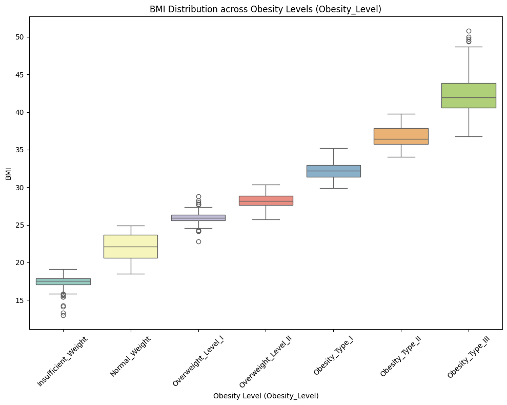
Observation:
✅ BMI increases consistently with obesity severity. Variability also rises at higher obesity levels, while normal and insufficient weight groups are more tightly distributed.
📈 BMI Distribution by Gender
# BMI distribution across different obesity levels (NObeyesdad)

plt.figure(figsize=(10,8))
sns.boxplot(x='Gender', y='BMI', data=data, palette='Set3')
plt.title('BMI Distribution by Gender')
plt.xlabel('Gender')
plt.ylabel('BMI')
plt.tight_layout()
plt.show()
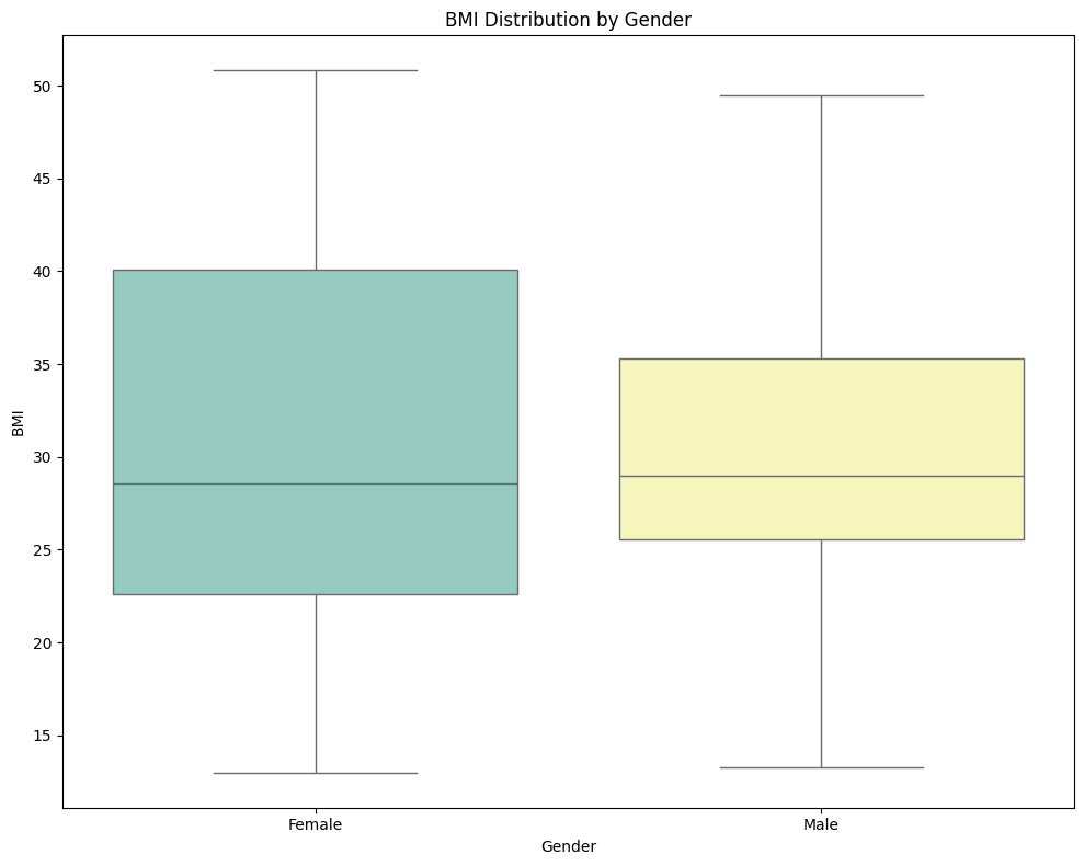
Observation:
✅ The plot shows that females, on average, tend to have a higher and more varied BMI compared to males. The broader spread of BMI values in females suggests more diversity in body composition within this group.</span>
plt.figure(figsize=(15,6))
ax = sns.countplot(x = "Gender", hue = "Obesity_Level",hue_order=nobeyesdad_order, data = data, palette='Set3')

for p in ax.patches:
    ax.annotate(format(p.get_height(), '.0f'),
               (p.get_x() + p.get_width() / 2, p.get_height()),
               ha = 'center', va = 'center',
               xytext = (0,10),
               textcoords = 'offset points')

plt.title("Distribution of Obesity_Level across Gender")
plt.xlabel('')
plt.ylabel('')

plt.show()
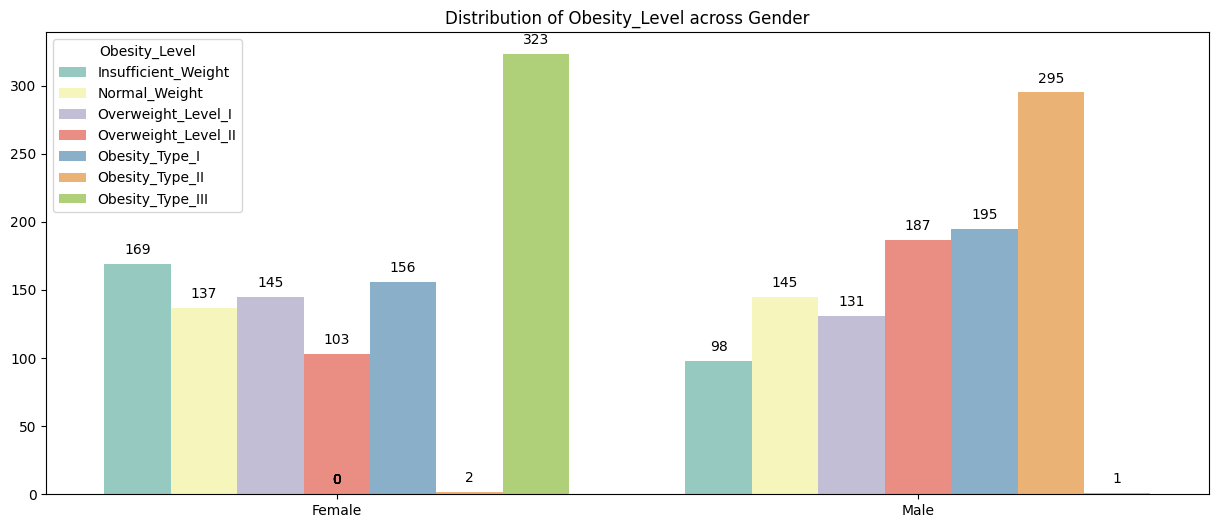
Observation:
✅ Females exhibit a wider and higher range of BMI values than males, indicating greater variability in body composition.
📈 BMI Distribution by Age
plt.figure(figsize=(10,8))
sns.scatterplot(x='Age', y='BMI', data=data, hue_order= nobeyesdad_order,hue='Obesity_Level', palette='Set3')

plt.title('BMI Distribution by Age')
plt.xlabel('Age')
plt.ylabel('BMI')
plt.tight_layout()
plt.show()
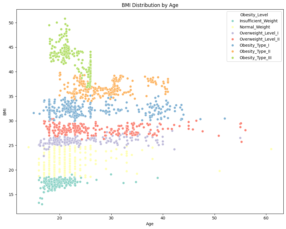
Observation:
✅ Obesity type III is more commonly observed in individuals under the age of 30. </span>
nobe_bmi_mean = data.groupby('Obesity_Level')['Age'].mean().reset_index()

nobe_bmi_mean_sorted = nobe_bmi_mean.sort_values(by='Age', ascending = False)

fig, axes = plt.subplots(1,2,figsize=(15,6))
sns.barplot(y='Obesity_Level', x='Age',ax=axes[0],data=nobe_bmi_mean,order=nobe_bmi_mean_sorted['Obesity_Level'],palette='Set3')

for index, row in enumerate(nobe_bmi_mean_sorted.iterrows()):
    axes[0].text(row[1]['Age'], index, f"{row[1]['Age']: .2f}", va = 'center', ha = 'left', fontsize = 10)

axes[0].set_xlabel('Age')
axes[0].set_ylabel('')
axes[0].set_xticklabels(axes[0].get_xticklabels(), rotation=45)

sns.violinplot(y = "Obesity_Level", x= "Age", data= data, ax=axes[1], order=nobe_bmi_mean_sorted['Obesity_Level'],palette='Set3')
axes[1].set_ylabel('')
axes[1].set_yticklabels([])

fig.suptitle('Average Age by NObeyesdad', fontsize = 16)
plt.show()
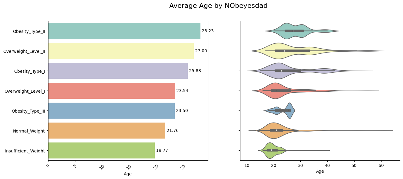
Observation:
✅ Normal Weight or Insufficient weight people seems to be younger on an average than the rest </span>
📈 BMI Distribution by Family History with Overweight
# Plot BMI distribution by Family History with Overweight across Obesity Levels
binary_palette = {"yes": "#8dd3c7", "no": "#fb8072"}

plt.figure(figsize=(12, 8))
sns.boxplot(
    x='Obesity_Level',
    y='BMI',
    hue ='Family_History',
    data=data,
    palette= binary_palette,
    order=obesity_level_order
)
plt.title("BMI Distribution by Family History with Overweight Across Obesity Levels", fontsize=16)
plt.xlabel("Obesity Level")
plt.ylabel("BMI")
plt.xticks(rotation=45)
plt.legend(title="Family History", loc='upper left')
plt.tight_layout()
plt.show()
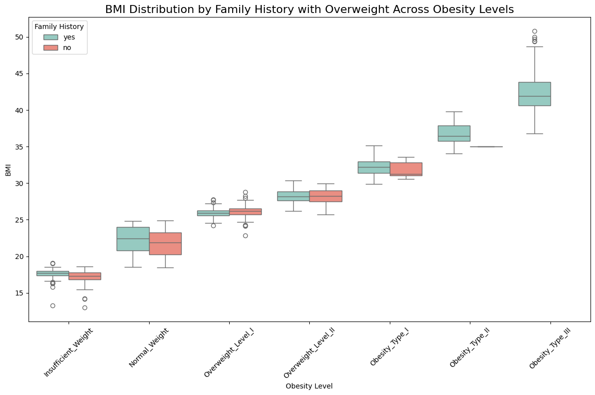
Observation:
✅ There is a strong evidence higher BMI levels have a family history of obesity.
✅ No cases of obesity level III have been observed in individuals without a family history of overweight, suggesting that family history plays a significant role, at least in the development of obesity level III. </span>
📈 BMI Distribution by Frequent Consumption of High-Calorie Food (FAVC)
# Plot BMI distribution by Family History with Overweight across Obesity Levels
binary_palette = {"yes": "#8dd3c7", "no": "#fb8072"}

plt.figure(figsize=(12, 8))
sns.boxplot(
    x='Obesity_Level',
    y='BMI',
    hue ='High_Cal_Foods_Frequently',
    data=data,
    palette= binary_palette,
    order=obesity_level_order
)
plt.title("BMI Distribution by Frequent Consumption of High-Calorie Food (FAVC)", fontsize=16)
plt.xlabel("Obesity Level")
plt.ylabel("BMI")
plt.xticks(rotation=45)
plt.legend(title="High_Cal_Foods_Frequently", loc='upper left')
plt.tight_layout()
plt.show()
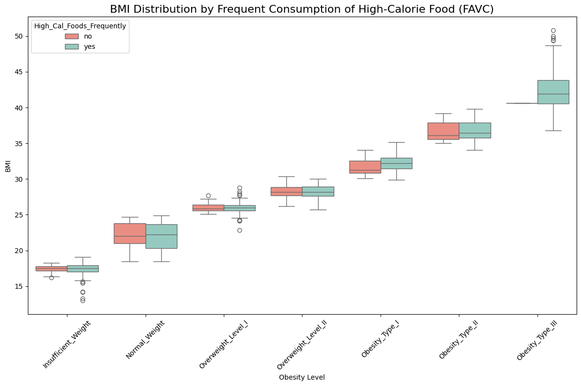
Observation:
✅ There is only one case of Obesity Type III where frequent consumption of high-calorie food is not present, suggesting that frequent consumption of high-calorie food likely plays a key role in the development of Obesity Type III. For other types of obesity and normal weight individuals, the distribution of high-calorie food consumption appears to be similar across all levels.
📈 BMI Distribution by Number of Meals (NCP)
# BMI distribution by Number of Meals (NCP) across different obesity levels (NObeyesdad)

plt.figure(figsize=(10,8))
sns.scatterplot(x='Num_Meals', y='BMI', data=obesity_df_renamed, hue='Obesity_Level', palette='Set3')

plt.title('BMI Distribution by Number of Meals (NCP)')
plt.xlabel('Number of Meals (NCP)')
plt.ylabel('BMI')
plt.tight_layout()
plt.show()
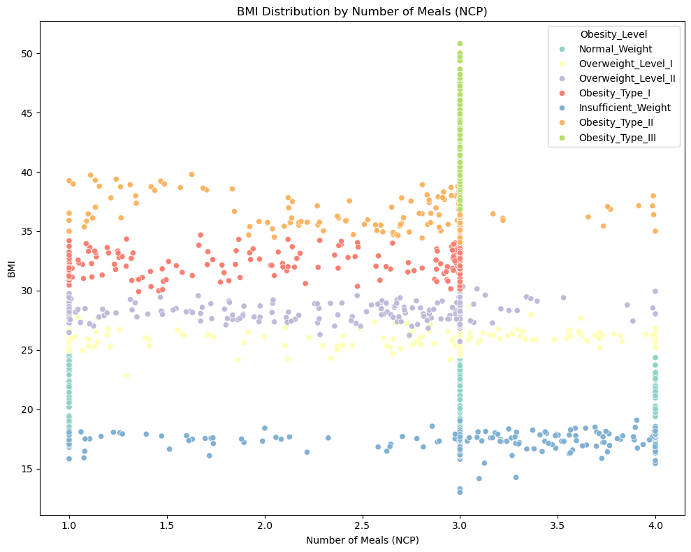
Observation:
✅ Obestiy type III are mostly consuming 3 meals where as normal weight people are consuming 1, 3 or 4 meals </span>
📈 BMI Distribution by Smoking Habit (SMOKE)
# Plot BMI distribution by Smoking across Obesity Levels
binary_palette = {"yes": "#8dd3c7", "no": "#fb8072"}

plt.figure(figsize=(12, 8))
sns.boxplot(
    x='Obesity_Level',
    y='BMI',
    hue ='Smoke',
    data=data,
    palette= binary_palette,
    order=obesity_level_order
)
plt.title("BMI Distribution by Smoking Habit ", fontsize=16)
plt.xlabel("Obesity Level")
plt.ylabel("BMI")
plt.xticks(rotation=45)
plt.legend(title="smoking", loc='upper left')
plt.tight_layout()
plt.show()
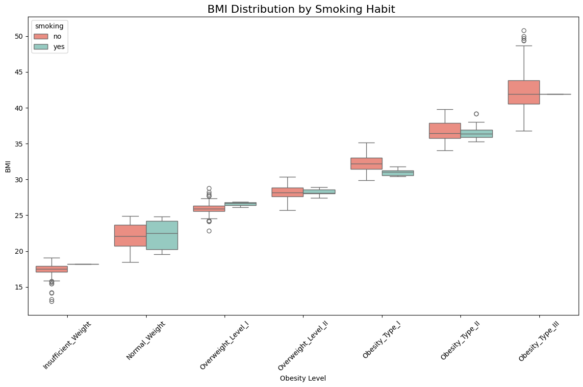
Observation:
✅ There is insufficient evidence to conclude that smoking has a significant effect on obesity levels. The primary observation is that individuals in Obesity Level III are predominantly non-smokers.
def show_pie_chart(df, column_name):

    # Converting string values to categorical
    df[column_name] = df[column_name].astype('category')

    # Calculating the frequency of values in the column
    counts = df[column_name].value_counts()


    # Sorting the values in the column by their frequency in descending order
    counts_sorted = counts.sort_values(ascending=False)

    # subplot
    fig,axes = plt.subplots(1, 2, figsize=(16, 8))
    plt.title(column_name)
    plt.subplots_adjust(wspace = 0.5)


    axes[0].pie(counts.values, labels=counts_sorted.index, autopct='%1.1f%%', startangle=140, colors=sns.color_palette("pastel"))

    sns.countplot(data=df, y=column_name, ax=axes[1], order=counts_sorted.index, palette="pastel", hue=column_name, legend=False, width=0.8)
    axes[1].set_ylabel('')
    axes[1].set_xlabel('')

    for i, v in enumerate(counts_sorted.values):
        axes[1].text(v + 0.1, i, str(v), ha='left', va = 'center', color = 'black', fontweight = 'bold')
    #plt.title(column_name)
    plt.show()
📈 BMI Distribution by Public Transportation (MTRANS)
 #Create pie chart for MTRANS
show_pie_chart(data, 'Transportation')
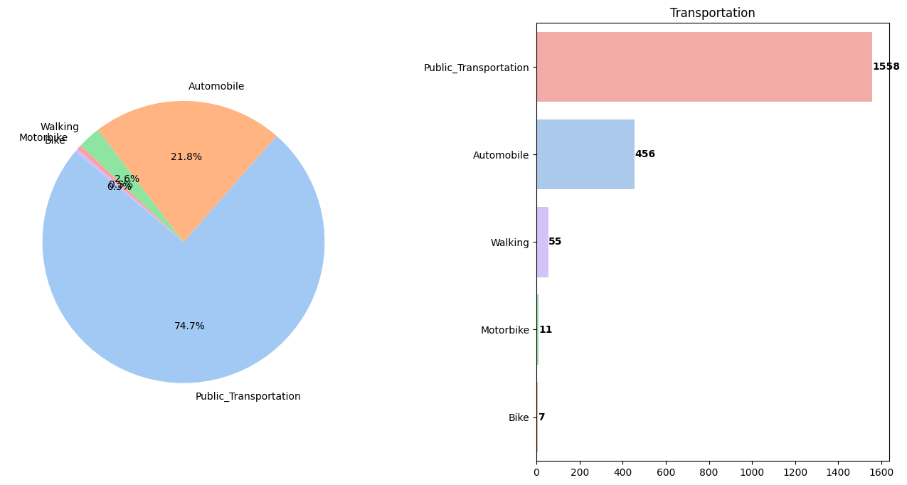
Observation:
✅ 97.6% use some form of vehicles while only ~2.7% prefers walking/using bike That’s concerning!</span>
📦 Export Cleaned Dataset
data.to_csv('clean_data.csv', index=False)
📌 Summary
- Obesity_Type I has the highest number of individuals.
- Most individuals have a family history of obesity.
- ~2.7% prefer walking/biking; the rest use vehicles — a concerning imbalance.
- More females are classified as obese compared to males.
- Strong positive correlation observed between Weight and Height.
- Outliers present in Age distribution.
🤖 Obesity Estimation - Feature Engineering & ML Models
We apply multiple classification models to identify the best-performing model for predicting obesity levels.
🧠 Models Considered
- Decision Tree
- Random Forest
- K-Nearest Neighbors (KNN)
- XGBoost (XGBClassifier)
🧭 Workflow Steps
- Train-Test Split (Stratified)
- One-Hot Encoding (categorical features)
- Standard Scaling (numerical features)
- Label Encoding (target variable)
- GridSearchCV + 5-Fold CV for performance tuning
- Feature Importance Analysis
🔍 Load and Preprocess Data
import pandas as pd

clean_data_df = pd.read_csv(r'../data/clean_data.csv')

clean_data_df.info()
clean_data_df.drop('BMI', axis='columns', inplace=True)
<class 'pandas.core.frame.DataFrame'>
RangeIndex: 2087 entries, 0 to 2086
Data columns (total 18 columns):
 #   Column                     Non-Null Count  Dtype
---  ------                     --------------  -----
 0   Gender                     2087 non-null   object
 1   Age                        2087 non-null   float64
 2   Height                     2087 non-null   float64
 3   Weight                     2087 non-null   float64
 4   Family_History             2087 non-null   object
 5   High_Cal_Foods_Frequently  2087 non-null   object
 6   Freq_Veg                   2087 non-null   float64
 7   Num_Meals                  2087 non-null   float64
 8   Snacking                   2087 non-null   object
 9   Smoke                      2087 non-null   object
 10  Water_Intake               2087 non-null   float64
 11  Calorie_Monitoring         2087 non-null   object
 12  Phys_Activity              2087 non-null   float64
 13  Tech_Use                   2087 non-null   float64
 14  Freq_Alcohol               2087 non-null   object
 15  Transportation             2087 non-null   object
 16  Obesity_Level              2087 non-null   object
 17  BMI                        2087 non-null   float64
dtypes: float64(9), object(9)
memory usage: 293.6+ KB
🧾 Identify Feature Types
cat_cols = ['Gender', 'Family_History', 'High_Cal_Foods_Frequently', 'Snacking','Smoke', 'Calorie_Monitoring', 'Freq_Alcohol', 'Transportation']

num_cols = ['Age', 'Height', 'Weight', 'Freq_Veg', 'Num_Meals','Water_Intake', 'Phys_Activity', 'Tech_Use']
🎯 Define Feature Matrix X and Target y
X = clean_data_df.drop('Obesity_Level',axis=1)
y = clean_data_df['Obesity_Level']

X.shape, y.shape
((2087, 16), (2087,))
🔄 Stratified Train-Test Split
Stratified splitting means that when you generate a training / validation dataset split, it will attempt to keep the same percentages of classes in each split.
These dataset divisions are usually generated randomly according to a target variable. However, when doing so, the proportions of the target variable among the different splits can differ, especially in the case of small datasets.
from sklearn.model_selection import train_test_split

X_train,X_test,y_train,y_test=train_test_split(X,y,stratify=y,test_size=0.2,random_state=42)

X_train.shape, X_test.shape, y_train.shape, y_test.shape
((1669, 16), (418, 16), (1669,), (418,))
⚙️ Preprocessing: One-Hot Encoding + Standard Scaling
from sklearn.preprocessing import OneHotEncoder
from sklearn.compose import make_column_transformer
from sklearn.preprocessing import StandardScaler
Sscaler = StandardScaler().set_output(transform="pandas")
# Encoding multiple columns.
transformer = make_column_transformer((Sscaler, num_cols), (OneHotEncoder(handle_unknown='ignore'),
     cat_cols),verbose=True,verbose_feature_names_out=True, remainder='drop')

transformer
ColumnTransformer(transformers=[('standardscaler', StandardScaler(),
                                 ['Age', 'Height', 'Weight', 'Freq_Veg',
                                  'Num_Meals', 'Water_Intake', 'Phys_Activity',
                                  'Tech_Use']),
                                ('onehotencoder',
                                 OneHotEncoder(handle_unknown='ignore'),
                                 ['Gender', 'Family_History',
                                  'High_Cal_Foods_Frequently', 'Snacking',
                                  'Smoke', 'Calorie_Monitoring', 'Freq_Alcohol',
                                  'Transportation'])],
                  verbose=True)
In a Jupyter environment, please rerun this cell to show the HTML representation or trust the notebook. On GitHub, the HTML representation is unable to render, please try loading this page with nbviewer.org.
ColumnTransformer(transformers=[('standardscaler', StandardScaler(),
                                 ['Age', 'Height', 'Weight', 'Freq_Veg',
                                  'Num_Meals', 'Water_Intake', 'Phys_Activity',
                                  'Tech_Use']),
                                ('onehotencoder',
                                 OneHotEncoder(handle_unknown='ignore'),
                                 ['Gender', 'Family_History',
                                  'High_Cal_Foods_Frequently', 'Snacking',
                                  'Smoke', 'Calorie_Monitoring', 'Freq_Alcohol',
                                  'Transportation'])],
verbose=True)['Age', 'Height', 'Weight', 'Freq_Veg', 'Num_Meals', 'Water_Intake', 'Phys_Activity', 'Tech_Use']
StandardScaler()
['Gender', 'Family_History', 'High_Cal_Foods_Frequently', 'Snacking', 'Smoke', 'Calorie_Monitoring', 'Freq_Alcohol', 'Transportation']
OneHotEncoder(handle_unknown='ignore')
🔄 X_train Encoding
# Transforming
transformed = transformer.fit_transform(X_train)
# Transformating back
transformed_df = pd.DataFrame(transformed, columns=transformer.get_feature_names_out())
# One-hot encoding removed an index. Let's put it back:
transformed_df.index = X_train.index
# Joining tables
X_train = pd.concat([X_train, transformed_df], axis=1)
# Dropping old categorical columns
X_train.drop(cat_cols, axis=1, inplace=True)
# Dropping old num columns
X_train.drop(num_cols, axis=1, inplace=True)
# CHecking result
#print(X_train.head())
print(X_train.columns)
print(X_train.shape)
[ColumnTransformer]  (1 of 2) Processing standardscaler, total=   0.0s
[ColumnTransformer] . (2 of 2) Processing onehotencoder, total=   0.0s
Index(['standardscaler__Age', 'standardscaler__Height',
       'standardscaler__Weight', 'standardscaler__Freq_Veg',
       'standardscaler__Num_Meals', 'standardscaler__Water_Intake',
       'standardscaler__Phys_Activity', 'standardscaler__Tech_Use',
       'onehotencoder__Gender_Female', 'onehotencoder__Gender_Male',
       'onehotencoder__Family_History_no', 'onehotencoder__Family_History_yes',
       'onehotencoder__High_Cal_Foods_Frequently_no',
       'onehotencoder__High_Cal_Foods_Frequently_yes',
       'onehotencoder__Snacking_Always', 'onehotencoder__Snacking_Frequently',
       'onehotencoder__Snacking_Sometimes', 'onehotencoder__Snacking_no',
       'onehotencoder__Smoke_no', 'onehotencoder__Smoke_yes',
       'onehotencoder__Calorie_Monitoring_no',
       'onehotencoder__Calorie_Monitoring_yes',
       'onehotencoder__Freq_Alcohol_Always',
       'onehotencoder__Freq_Alcohol_Frequently',
       'onehotencoder__Freq_Alcohol_Sometimes',
       'onehotencoder__Freq_Alcohol_no',
       'onehotencoder__Transportation_Automobile',
       'onehotencoder__Transportation_Bike',
       'onehotencoder__Transportation_Motorbike',
       'onehotencoder__Transportation_Public_Transportation',
       'onehotencoder__Transportation_Walking'],
      dtype='object')
      ```

(1669, 31)
🔄 X_test Encoding
# Transforming
transformed = transformer.transform(X_test)
# Transformating back
transformed_df = pd.DataFrame(transformed, columns=transformer.get_feature_names_out())
# One-hot encoding removed an index. Let's put it back:
transformed_df.index = X_test.index
# Joining tables
X_test = pd.concat([X_test, transformed_df], axis=1)
# Dropping old categorical columns
X_test.drop(cat_cols, axis=1, inplace=True)
# Dropping old num columns
X_test.drop(num_cols, axis=1, inplace=True)
# CHecking result
X_test.head()
| standardscaler__Age | standardscaler__Height | standardscaler__Weight | standardscaler__Freq_Veg | standardscaler__Num_Meals | standardscaler__Water_Intake | standardscaler__Phys_Activity | standardscaler__Tech_Use | onehotencoder__Gender_Female | onehotencoder__Gender_Male | ... | onehotencoder__Calorie_Monitoring_yes | onehotencoder__Freq_Alcohol_Always | onehotencoder__Freq_Alcohol_Frequently | onehotencoder__Freq_Alcohol_Sometimes | onehotencoder__Freq_Alcohol_no | onehotencoder__Transportation_Automobile | onehotencoder__Transportation_Bike | onehotencoder__Transportation_Motorbike | onehotencoder__Transportation_Public_Transportation | onehotencoder__Transportation_Walking | |
|---|---|---|---|---|---|---|---|---|---|---|---|---|---|---|---|---|---|---|---|---|---|
| 1153 | -0.690071 | -1.202029 | -0.537291 | 1.084280 | 1.512030 | -0.000656 | 0.376859 | 0.550747 | 1.0 | 0.0 | ... | 0.0 | 0.0 | 0.0 | 1.0 | 0.0 | 0.0 | 0.0 | 0.0 | 1.0 | 0.0 |
| 132 | 0.899810 | 0.736866 | 0.848928 | 1.084280 | 0.391801 | -1.644954 | 1.182627 | -1.095082 | 0.0 | 1.0 | ... | 0.0 | 0.0 | 0.0 | 1.0 | 0.0 | 1.0 | 0.0 | 0.0 | 0.0 | 0.0 |
| 1923 | -0.587828 | 0.401573 | 1.579131 | 1.084280 | 0.391801 | -0.334381 | 0.499952 | 0.495086 | 1.0 | 0.0 | ... | 0.0 | 0.0 | 0.0 | 1.0 | 0.0 | 0.0 | 0.0 | 0.0 | 1.0 | 0.0 |
| 846 | -1.165664 | -1.047678 | -0.831968 | 1.008997 | -2.224232 | -0.000656 | -0.324357 | 1.117030 | 1.0 | 0.0 | ... | 1.0 | 0.0 | 0.0 | 0.0 | 1.0 | 0.0 | 0.0 | 0.0 | 1.0 | 0.0 |
| 1246 | 0.821665 | 1.347473 | 0.839435 | -0.801583 | 0.231677 | 0.588066 | -0.155934 | 1.895629 | 0.0 | 1.0 | ... | 0.0 | 0.0 | 0.0 | 1.0 | 0.0 | 1.0 | 0.0 | 0.0 | 0.0 | 0.0 |
5 rows × 31 columns
print(X_train.columns, X_train.shape)
Index(['standardscaler__Age', 'standardscaler__Height',
       'standardscaler__Weight', 'standardscaler__Freq_Veg',
       'standardscaler__Num_Meals', 'standardscaler__Water_Intake',
       'standardscaler__Phys_Activity', 'standardscaler__Tech_Use',
       'onehotencoder__Gender_Female', 'onehotencoder__Gender_Male',
       'onehotencoder__Family_History_no', 'onehotencoder__Family_History_yes',
       'onehotencoder__High_Cal_Foods_Frequently_no',
       'onehotencoder__High_Cal_Foods_Frequently_yes',
       'onehotencoder__Snacking_Always', 'onehotencoder__Snacking_Frequently',
       'onehotencoder__Snacking_Sometimes', 'onehotencoder__Snacking_no',
       'onehotencoder__Smoke_no', 'onehotencoder__Smoke_yes',
       'onehotencoder__Calorie_Monitoring_no',
       'onehotencoder__Calorie_Monitoring_yes',
       'onehotencoder__Freq_Alcohol_Always',
       'onehotencoder__Freq_Alcohol_Frequently',
       'onehotencoder__Freq_Alcohol_Sometimes',
       'onehotencoder__Freq_Alcohol_no',
       'onehotencoder__Transportation_Automobile',
       'onehotencoder__Transportation_Bike',
       'onehotencoder__Transportation_Motorbike',
       'onehotencoder__Transportation_Public_Transportation',
       'onehotencoder__Transportation_Walking'],
      dtype='object') (1669, 31)
# Setting new feature names

X_train.columns = ['Age', 'Height', 'Weight', 'Freq_Veg', 'Num_Meals', 'Water_Intake',
       'Phys_Activity', 'Tech_Use', 'Gender_Female',
       'Gender_Male', 'Family_History_no',
       'Family_History_yes',
       'High_Cal_Foods_Frequently_no',
       'High_Cal_Foods_Frequently_yes',
       'Snacking_Always', 'Snacking_Frequently',
       'Snacking_Sometimes', 'Snacking_no',
       'Smoke_no', 'Smoke_yes',
       'Calorie_Monitoring_no',
       'Calorie_Monitoring_yes',
       'Freq_Alcohol_Always',
       'Freq_Alcohol_Frequently',
       'Freq_Alcohol_Sometimes',
       'Freq_Alcohol_no',
       'Transportation_Automobile',
       'Transportation_Bike',
       'Transportation_Motorbike',
       'Transportation_Public_Transportation',
       'Transportation_Walking']

X_test.columns = ['Age', 'Height', 'Weight', 'Freq_Veg', 'Num_Meals', 'Water_Intake',
       'Phys_Activity', 'Tech_Use', 'Gender_Female',
       'Gender_Male', 'Family_History_no',
       'Family_History_yes',
       'High_Cal_Foods_Frequently_no',
       'High_Cal_Foods_Frequently_yes',
       'Snacking_Always', 'Snacking_Frequently',
       'Snacking_Sometimes', 'Snacking_no',
       'Smoke_no', 'Smoke_yes',
       'Calorie_Monitoring_no',
       'Calorie_Monitoring_yes',
       'Freq_Alcohol_Always',
       'Freq_Alcohol_Frequently',
       'Freq_Alcohol_Sometimes',
       'Freq_Alcohol_no',
       'Transportation_Automobile',
       'Transportation_Bike',
       'Transportation_Motorbike',
       'Transportation_Public_Transportation',
       'Transportation_Walking']
# After renaming the columns

X_train.head()
| Age | Height | Weight | Freq_Veg | Num_Meals | Water_Intake | Phys_Activity | Tech_Use | Gender_Female | Gender_Male | ... | Calorie_Monitoring_yes | Freq_Alcohol_Always | Freq_Alcohol_Frequently | Freq_Alcohol_Sometimes | Freq_Alcohol_no | Transportation_Automobile | Transportation_Bike | Transportation_Motorbike | Transportation_Public_Transportation | Transportation_Walking | |
|---|---|---|---|---|---|---|---|---|---|---|---|---|---|---|---|---|---|---|---|---|---|
| 1549 | 0.248290 | 0.705537 | 1.045026 | -0.375885 | 0.391801 | 0.253102 | 0.308538 | -0.452916 | 0.0 | 1.0 | ... | 0.0 | 0.0 | 0.0 | 1.0 | 0.0 | 0.0 | 0.0 | 0.0 | 1.0 | 0.0 |
| 1574 | 1.008501 | -0.608067 | 0.505277 | 1.016483 | -0.755149 | -1.644954 | 0.823971 | -0.073903 | 0.0 | 1.0 | ... | 0.0 | 0.0 | 0.0 | 0.0 | 1.0 | 0.0 | 0.0 | 0.0 | 1.0 | 0.0 |
| 1155 | 3.702329 | 0.457500 | -0.078269 | 0.207948 | 0.391801 | -1.403908 | -0.827757 | -1.095082 | 0.0 | 1.0 | ... | 0.0 | 0.0 | 0.0 | 0.0 | 1.0 | 1.0 | 0.0 | 0.0 | 0.0 | 0.0 |
| 610 | -0.208354 | 0.416482 | -1.265285 | -0.345947 | 0.391801 | -0.252848 | 1.731352 | 0.245475 | 1.0 | 0.0 | ... | 0.0 | 0.0 | 0.0 | 0.0 | 1.0 | 0.0 | 0.0 | 0.0 | 1.0 | 0.0 |
| 906 | -0.523216 | -1.012212 | -0.725998 | -0.801583 | 0.596256 | 1.643643 | 0.204484 | -0.952112 | 1.0 | 0.0 | ... | 0.0 | 0.0 | 0.0 | 1.0 | 0.0 | 0.0 | 0.0 | 0.0 | 1.0 | 0.0 |
5 rows × 31 columns
🧬 Apply Label Encoder
🔡 Encoding y_train
from sklearn.preprocessing import LabelEncoder

le = LabelEncoder()
y_train_encoded = le.fit_transform(y_train)

#y_train.head(10) , y_train_encoded[0:10]
🔡 Encoding y_test
le_test = LabelEncoder()
y_test_encoded = le_test.fit_transform(y_test)
y_test.head(10) , y_test_encoded[0:10]
(1153    Overweight_Level_II
 132          Obesity_Type_I
 1923       Obesity_Type_III
 846      Overweight_Level_I
 1246         Obesity_Type_I
 1236         Obesity_Type_I
 1372         Obesity_Type_I
 1010    Overweight_Level_II
 337        Obesity_Type_III
 1524        Obesity_Type_II
 Name: Obesity_Level, dtype: object,
 array([6, 2, 4, 5, 2, 2, 2, 6, 4, 3]))
🤖 Classifier Models
from sklearn.ensemble import RandomForestClassifier
from sklearn.tree import DecisionTreeClassifier
from sklearn.neighbors import KNeighborsClassifier
from xgboost import XGBClassifier
🧰 Models in Consideration
models={'RandomForest':RandomForestClassifier(),
        'DecisionTree':DecisionTreeClassifier(),
        'KNeighbors':KNeighborsClassifier(),
        'xgbc': XGBClassifier()}
🧪 Scoring for Measuring Model Performance
from sklearn.metrics import make_scorer, precision_score, recall_score, f1_score
scoring = {
    'accuracy': 'accuracy',
    'precision': make_scorer(precision_score, average='weighted'),
    'recall': make_scorer(recall_score, average='weighted'),
    'f1': make_scorer(f1_score, average='weighted')}
🧾 Model Evaluation
# %load ../models/Models_eval.py

from sklearn.model_selection import GridSearchCV

def grid_search_cv_eval(X,Y, models, param_grid, scorings,cross_validation):
    """Here we evaluate the models using gridsearchcv and returns the dictionary of best models and result."""

    best_models = {}
    result = {}
    print(models)
    for model in models:
        print(result)
        print(f"\nRunning GridSearch for {model}...")
        gsv = GridSearchCV(
            estimator=models[model],
            param_grid=param_grid[model],
            cv=cross_validation,
            scoring=scorings,
            refit='accuracy'  # Primary metric for model selection
        )
        gsv.fit(X, Y)
        best_models[model] = gsv.best_estimator_
        best_index = gsv.best_index_
        print(f'Best parameters for {model}: {gsv.best_params_}')
        print(f'Best accuracy: {gsv.cv_results_["mean_test_accuracy"][best_index]:.4f}')
        print(f'Best precision: {gsv.cv_results_["mean_test_precision"][best_index]:.4f}')
        print(f'Best recall: {gsv.cv_results_["mean_test_recall"][best_index]:.4f}')
        result[model] = {"parameter":gsv.best_params_,"accuracy":gsv.cv_results_["mean_test_accuracy"][best_index], "precision": gsv.cv_results_["mean_test_precision"][best_index],"recall": gsv.cv_results_["mean_test_recall"][best_index]}

    return best_models, result


from sklearn.model_selection import cross_val_score

# Define the function to compare models with default parameters
def evaluate_models(X, Y, models, scorings, cross_validation):
    result = {}

    # Loop through models and evaluate each one
    for model_name, model in models.items():
        print(f"\nEvaluating {model_name}...")

        # Evaluate using the defined scoring metrics
        model_scores = {}
        for score_name, scorer in scorings.items():
            score = cross_val_score(model, X, Y, cv=cross_validation, scoring=scorer)
            model_scores[score_name] = score.mean()

        # Store results
        result[model_name] = model_scores

        # Print the results
        print(f"Accuracy: {model_scores['accuracy']:.4f}")
        print(f"Precision: {model_scores['precision']:.4f}")
        print(f"Recall: {model_scores['recall']:.4f}")
        print(f"F1 Score: {model_scores['f1']:.4f}")

    return result

result = evaluate_models(X_train, y_train_encoded, models, scoring, 5)
Evaluating RandomForest...
Accuracy: 0.9323
Precision: 0.9389
Recall: 0.9341
F1 Score: 0.9352

Evaluating DecisionTree...
Accuracy: 0.9191
Precision: 0.9230
Recall: 0.9167
F1 Score: 0.9180

Evaluating KNeighbors...
Accuracy: 0.8113
Precision: 0.8105
Recall: 0.8113
F1 Score: 0.7941

Evaluating xgbc...
Accuracy: 0.9629
Precision: 0.9633
Recall: 0.9629
F1 Score: 0.9628
📊 Models Performance Visuals
result_df = pd.DataFrame(result).T
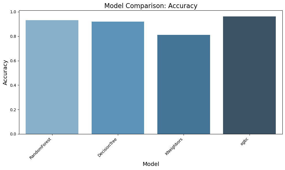
📈 Accuracy Comparison
# Plot Accuracy
import matplotlib.pyplot as plt
import seaborn as sns
plt.figure(figsize=(10, 6))
sns.barplot(x=result_df.index, y='accuracy', data=result_df, palette="Blues_d")
plt.title('Model Comparison: Accuracy', fontsize=16)
plt.ylabel('Accuracy', fontsize=14)
plt.xlabel('Model', fontsize=14)
plt.xticks(rotation=45, ha='right')
plt.tight_layout()
plt.show()
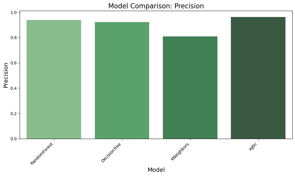
🎯 Precision Comparison
# Plot Precision
plt.figure(figsize=(10, 6))
sns.barplot(x=result_df.index, y='precision', data=result_df, palette="Greens_d")
plt.title('Model Comparison: Precision', fontsize=16)
plt.ylabel('Precision', fontsize=14)
plt.xlabel('Model', fontsize=14)
plt.xticks(rotation=45, ha='right')
plt.tight_layout()
plt.show()
🔁 Recall Comparison
# Plot Precision
plt.figure(figsize=(10, 6))
sns.barplot(x=result_df.index, y='recall', data=result_df, palette="Oranges_d")
plt.title('Model Comparison: Recall', fontsize=16)
plt.ylabel('Recall', fontsize=14)
plt.xlabel('Model', fontsize=14)
plt.xticks(rotation=45, ha='right')
plt.tight_layout()
plt.show()
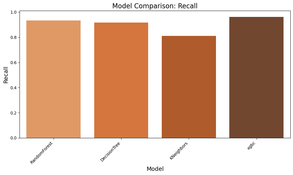
Observation:
✅ Based on Visuals above we can clearly notice that RandomForest and XGBC models are showing good results. We will tune the parameters next to find the best suitable model
📋 Creating a Comparison Table for the Models
models = ['RandomForest', 'DecisionTree', 'KNeighbors', 'xgbc']

result_df['f1_score'] = 2 * (result_df['precision'] * result_df['recall']) / (result_df['precision'] + result_df['recall'])

# Display the updated table with F1 score
display(result_df)
| accuracy | precision | recall | f1 | f1_score | |
|---|---|---|---|---|---|
| RandomForest | 0.932303 | 0.938914 | 0.934096 | 0.935160 | 0.936499 |
| DecisionTree | 0.919117 | 0.923018 | 0.916723 | 0.917965 | 0.919860 |
| KNeighbors | 0.811273 | 0.810466 | 0.811273 | 0.794125 | 0.810869 |
| xgbc | 0.962854 | 0.963345 | 0.962854 | 0.962758 | 0.963100 |
Observation:
✅ The results highlight that the xgbc model outperforms others with the highest accuracy (96.3%), precision (96.3%), recall (96.3%), and F1 score (96.3%), demonstrating its superior ability to classify data correctly. The RandomForest model also shows strong performance, achieving an accuracy of 93.7%, making it a competitive alternative. In comparison, the DecisionTree model and KNeighbors model perform slightly lower, with accuracies of 92.2% and 81.1%, respectively. Based on these findings, we have decided to conduct further comparisons between RandomForest and XGBoost to refine our model selection process.
⚙️ Hyperparameter Tuning: Random Forest & XGBoost
models={'RandomForest_hyper_tuned':RandomForestClassifier(),
        'xgbc_hyper_tuned': XGBClassifier()}

# Hyperparameter grids for tuning models
param_grids = {
    # Random Forest Hyperparameter Grid
    'RandomForest_hyper_tuned': {
        'n_estimators': [50, 100, 200, 400],               # Number of trees in the forest
        'max_depth': [None, 10, 20, 50],                   # Maximum depth of each tree
        'min_samples_split': [2, 5, 10, 15]                # Minimum number of samples to split a node
    },
    # XGBoostClassifier Hyperparameter Grid
    'xgbc_hyper_tuned': {
        'n_estimators': [50, 100, 200, 400],               # Number of boosting rounds
        'max_depth': [3, 5, 7, 10],                        # Maximum depth of each tree
        'learning_rate': [0.001, 0.01, 0.1, 0.3],          # Step size shrinkage
        'objective': ['multi:softmax'],                    # Multi-class classification
        'verbosity': [0],                                  # Silence output
        'nthread': [-1],                                   # Use all available threads
        'random_state': [42]                               # Ensure reproducibility
    }
}

best_models_hyper_tuned, result_hyper_tuned = grid_search_cv_eval(X_train, y_train_encoded, models, param_grids, scoring, cross_validation=5)
best_models_hyper_tuned, result_hyper_tuned
{'RandomForest_hyper_tuned': RandomForestClassifier(), 'xgbc_hyper_tuned': XGBClassifier(base_score=None, booster=None, callbacks=None,
              colsample_bylevel=None, colsample_bynode=None,
              colsample_bytree=None, device=None, early_stopping_rounds=None,
              enable_categorical=False, eval_metric=None, feature_types=None,
              gamma=None, grow_policy=None, importance_type=None,
              interaction_constraints=None, learning_rate=None, max_bin=None,
              max_cat_threshold=None, max_cat_to_onehot=None,
              max_delta_step=None, max_depth=None, max_leaves=None,
              min_child_weight=None, missing=nan, monotone_constraints=None,
              multi_strategy=None, n_estimators=None, n_jobs=None,
              num_parallel_tree=None, random_state=None, ...)}
{}

Running GridSearch for RandomForest_hyper_tuned...
Best parameters for RandomForest_hyper_tuned: {'max_depth': 50, 'min_samples_split': 5, 'n_estimators': 400}
Best accuracy: 0.9371
Best precision: 0.9424
Best recall: 0.9371
{'RandomForest_hyper_tuned': {'parameter': {'max_depth': 50, 'min_samples_split': 5, 'n_estimators': 400}, 'accuracy': 0.9370915826005646, 'precision': 0.9423907933895954, 'recall': 0.9370915826005646}}

Running GridSearch for xgbc_hyper_tuned...
Best parameters for xgbc_hyper_tuned: {'learning_rate': 0.1, 'max_depth': 5, 'n_estimators': 400, 'nthread': -1, 'objective': 'multi:softmax', 'random_state': 42, 'verbosity': 0}
Best accuracy: 0.9664
Best precision: 0.9668
Best recall: 0.9664


({'RandomForest_hyper_tuned': RandomForestClassifier(max_depth=50, min_samples_split=5, n_estimators=400),
  'xgbc_hyper_tuned': XGBClassifier(base_score=None, booster=None, callbacks=None,
                colsample_bylevel=None, colsample_bynode=None,
                colsample_bytree=None, device=None, early_stopping_rounds=None,
                enable_categorical=False, eval_metric=None, feature_types=None,
                gamma=None, grow_policy=None, importance_type=None,
                interaction_constraints=None, learning_rate=0.1, max_bin=None,
                max_cat_threshold=None, max_cat_to_onehot=None,
                max_delta_step=None, max_depth=5, max_leaves=None,
                min_child_weight=None, missing=nan, monotone_constraints=None,
                multi_strategy=None, n_estimators=400, n_jobs=None, nthread=-1,
                num_parallel_tree=None, ...)},
 {'RandomForest_hyper_tuned': {'parameter': {'max_depth': 50,
    'min_samples_split': 5,
    'n_estimators': 400},
   'accuracy': 0.9370915826005646,
   'precision': 0.9423907933895954,
   'recall': 0.9370915826005646},
  'xgbc_hyper_tuned': {'parameter': {'learning_rate': 0.1,
    'max_depth': 5,
    'n_estimators': 400,
    'nthread': -1,
    'objective': 'multi:softmax',
    'random_state': 42,
    'verbosity': 0},
   'accuracy': 0.9664472856089622,
   'precision': 0.9668094661210735,
   'recall': 0.9664472856089622}})
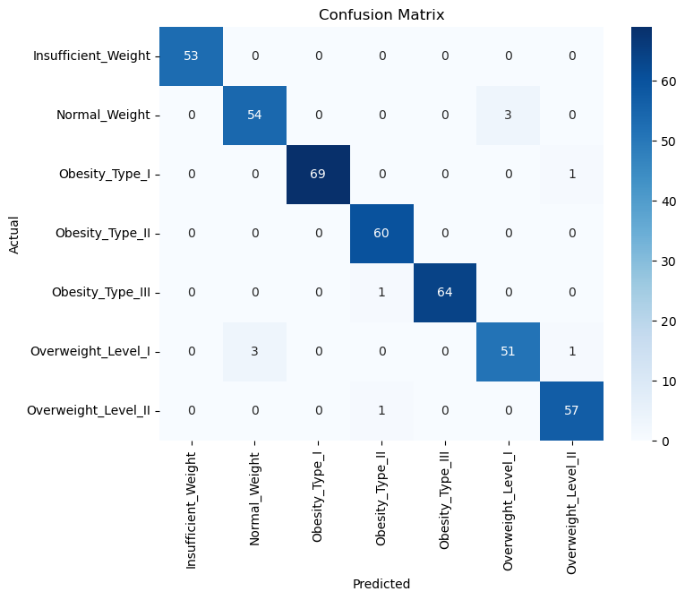
📉 Confusion Matrix
from sklearn.metrics import confusion_matrix
import seaborn as sns
import matplotlib.pyplot as plt

y_pred = best_models_hyper_tuned['xgbc_hyper_tuned'].predict(X_test)

cm = confusion_matrix(y_test_encoded, y_pred)

plt.figure(figsize=(8, 6))
sns.heatmap(cm, annot=True, fmt='d', cmap='Blues',
            xticklabels=le.classes_, yticklabels=le.classes_)
plt.xlabel('Predicted')
plt.ylabel('Actual')
plt.title('Confusion Matrix')
plt.show()
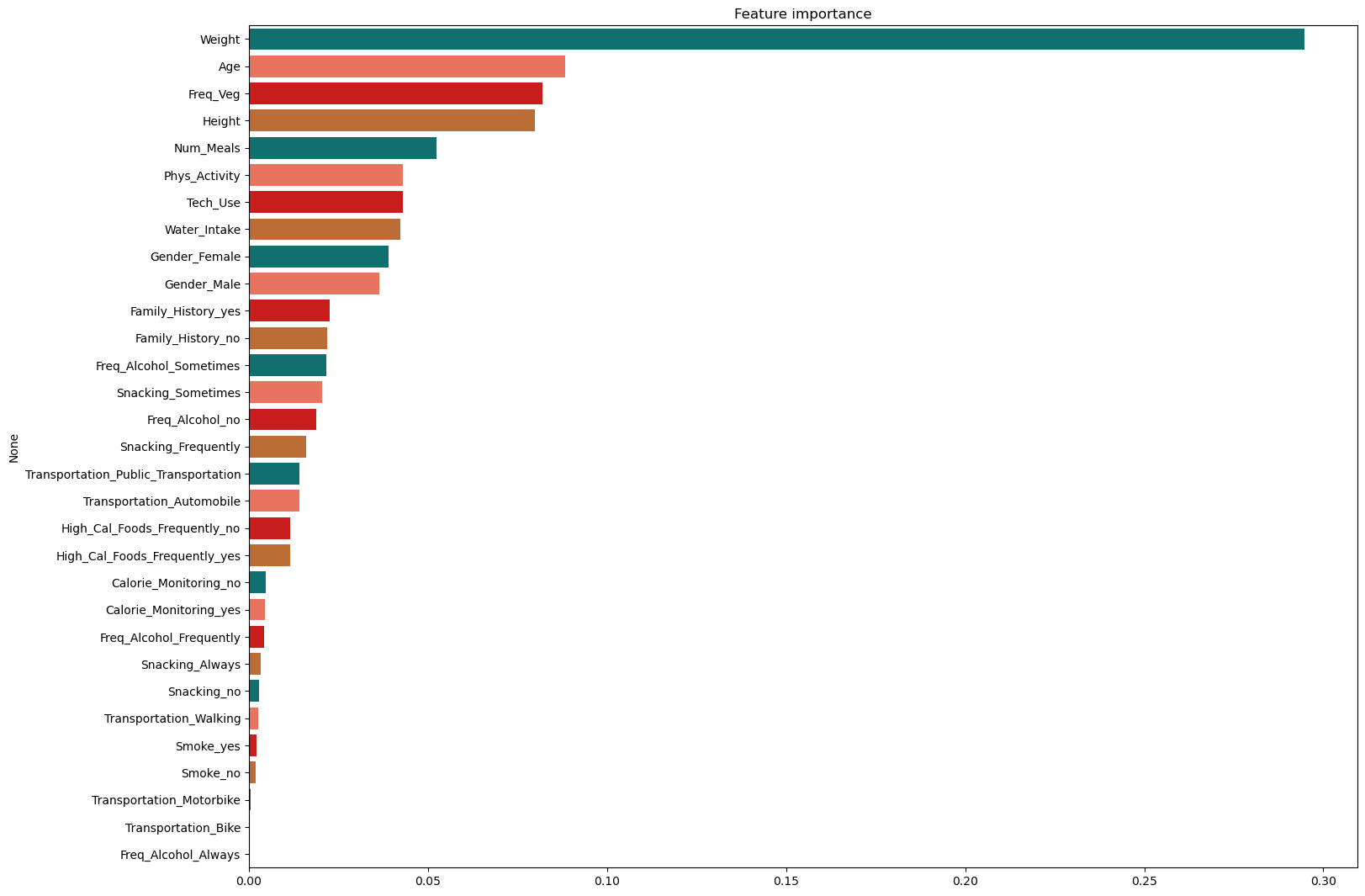
🌲 Feature Importance (Random Forest)
from sklearn.ensemble import RandomForestClassifier
import seaborn as sns
import plotly.express as px

from matplotlib import pyplot as plt
from sklearn.model_selection import cross_val_score

palette = ['#008080','#FF6347', '#E50000', '#D2691E'] # Creating color palette for plots

randomForest_model = best_models_hyper_tuned['RandomForest_hyper_tuned']
randomForest_model = randomForest_model.fit(X_train, y_train)

fimp = pd.Series(data=randomForest_model.feature_importances_, index=X_train.columns).sort_values(ascending=False)
plt.figure(figsize=(17,13))
plt.title("Feature importance")
ax = sns.barplot(y=fimp.index, x=fimp.values, palette=palette, orient='h')
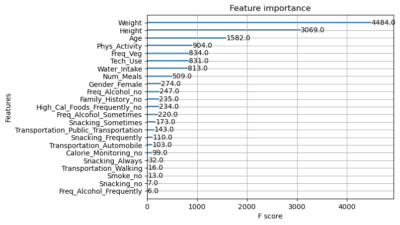
🎯 Classic Feature Attributions (XGBoost)
Here we try out the global feature importance calcuations that come with XGBoost.
xgboot_model = best_models_hyper_tuned.get('xgbc_hyper_tuned')
xgboot_model
XGBClassifier(base_score=None, booster=None, callbacks=None,
              colsample_bylevel=None, colsample_bynode=None,
              colsample_bytree=None, device=None, early_stopping_rounds=None,
              enable_categorical=False, eval_metric=None, feature_types=None,
              gamma=None, grow_policy=None, importance_type=None,
              interaction_constraints=None, learning_rate=0.1, max_bin=None,
              max_cat_threshold=None, max_cat_to_onehot=None,
              max_delta_step=None, max_depth=5, max_leaves=None,
              min_child_weight=None, missing=nan, monotone_constraints=None,
              multi_strategy=None, n_estimators=400, n_jobs=None, nthread=-1,
              num_parallel_tree=None, ...)
In a Jupyter environment, please rerun this cell to show the HTML representation or trust the notebook. On GitHub, the HTML representation is unable to render, please try loading this page with nbviewer.org.
XGBClassifier(base_score=None, booster=None, callbacks=None,
              colsample_bylevel=None, colsample_bynode=None,
              colsample_bytree=None, device=None, early_stopping_rounds=None,
              enable_categorical=False, eval_metric=None, feature_types=None,
              gamma=None, grow_policy=None, importance_type=None,
              interaction_constraints=None, learning_rate=0.1, max_bin=None,
              max_cat_threshold=None, max_cat_to_onehot=None,
              max_delta_step=None, max_depth=5, max_leaves=None,
              min_child_weight=None, missing=nan, monotone_constraints=None,
              multi_strategy=None, n_estimators=400, n_jobs=None, nthread=-1,
              num_parallel_tree=None, ...)
import xgboost
xgboost.plot_importance(xgboot_model)
#plt.title("xgboost plot_importance(model)")
plt.show()
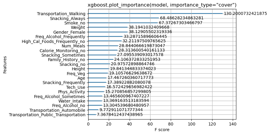
xgboost.plot_importance(xgboot_model, importance_type="cover")
plt.title('xgboost.plot_importance(model, importance_type="cover")')
plt.show()
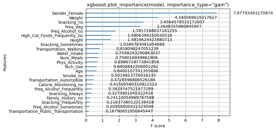
xgboost.plot_importance(xgboot_model, importance_type="gain")
plt.title('xgboost.plot_importance(model, importance_type="gain")')
plt.show()
🧠 SHAP Explainability Setup
import shap

# print the JS visualization code to the notebook
shap.initjs()

🧠 SHAP Explainability – TreeExplainer (XGBoost)
explainer = shap.TreeExplainer(xgboot_model)
shap_values = explainer.shap_values(X_train)
####📌 SHAP Summary Plot (All Features)
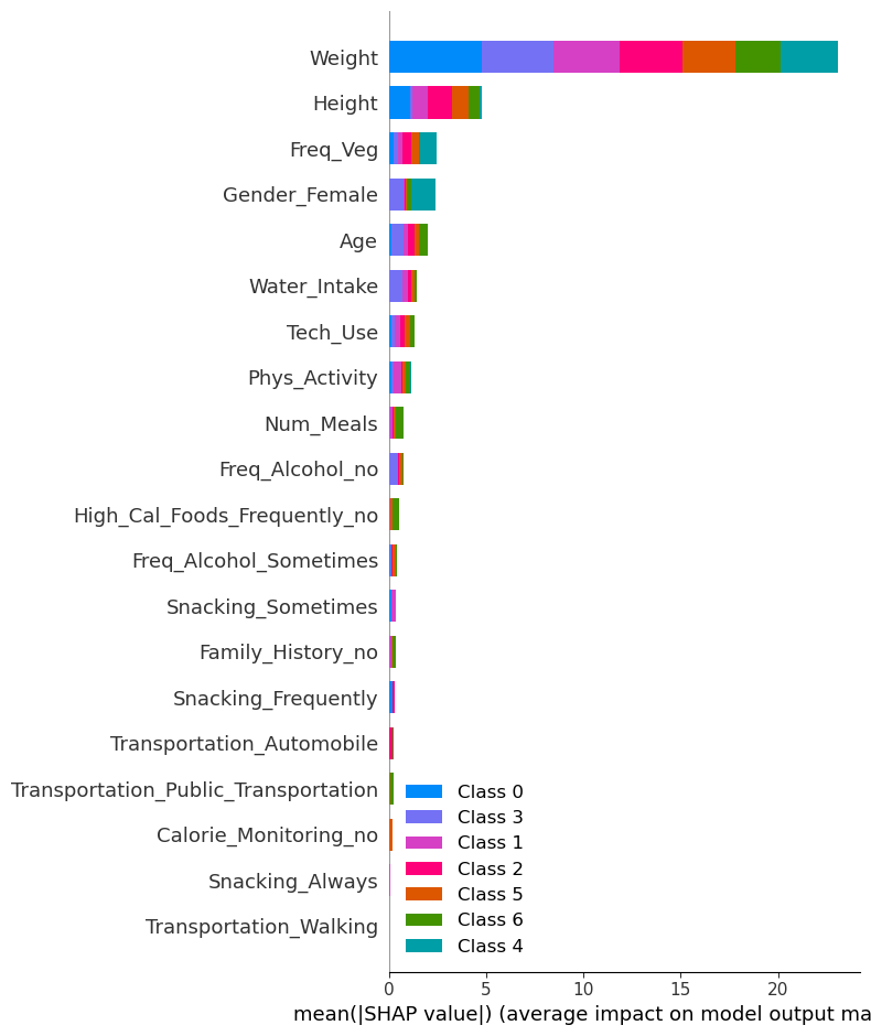
shap.summary_plot(shap_values, X_train, plot_type="bar")
!
class_mapping = {
    'Insufficient_Weight': 0,
    'Normal_Weight': 1,
    'Overweight_Level_I': 2,
    'Overweight_Level_II': 3,
    'Obesity_Type_I': 4,
    'Obesity_Type_II': 5,
    'Obesity_Type_III': 6
}
🧠 Feature Importance Insights
Top Features:
- Weight is the most dominant feature, influencing predictions across all classes substantially.
- Height and Freq_Veg also show strong predictive power across multiple obesity levels.
Lower Features:
- Features like Transportation_Walking, Snacking_Always, and Calorie_Monitoring_no contribute very little to predictions and may not add significant predictive power.
Class-Specific Observations:
- Weight and Height influence multiple classes, especially Class 0 (Insufficient_Weight) and Class 4 (Obesity_Type_I).
- Some features (e.g., Transportation_Public_Transportation) may have niche relevance to specific classes.
- Overall, feature contribution patterns are fairly consistent across obesity levels.
🛠️ Feature Engineering (Without Height & Weight)
To assess the true impact of lifestyle and behavioral factors on obesity prediction, we retrain the XGBoost model after removing Weight and Height from the dataset.
from sklearn.model_selection import train_test_split
from sklearn.preprocessing import MinMaxScaler, LabelEncoder
from sklearn.metrics import accuracy_score, precision_score, recall_score, f1_score

# Drop Weight and Height
dataset_cleaned = clean_data_df.drop(columns=['Weight', 'Height'])

#  Separate features and target variable
X_new = dataset_cleaned.drop(columns=['Obesity_Level'])
y_new = dataset_cleaned['Obesity_Level']

# Encode categorical target variable
le = LabelEncoder()
y_encoded_new = le.fit_transform(y)

# Split data into training and testing sets
X_train_new, X_test_new, y_train_new, y_test_new = train_test_split(X_new, y_encoded_new, stratify=y_encoded_new, test_size=0.2, random_state=42)

# One-Hot Encode Categorical Features
categorical_features = ['Gender', 'Family_History', 'High_Cal_Foods_Frequently', 'Snacking',
                        'Smoke', 'Calorie_Monitoring', 'Freq_Alcohol', 'Transportation']
X_train_new = pd.get_dummies(X_train_new, columns=categorical_features, drop_first=True)
X_test_new = pd.get_dummies(X_test_new, columns=categorical_features, drop_first=True)

# Ensure train and test datasets have the same columns
X_test_new = X_test_new.reindex(columns=X_train_new.columns, fill_value=0)

# Step 2: Apply Min-Max Scaling to Numerical Features
num_cols = ['Age', 'Freq_Veg', 'Num_Meals', 'Water_Intake', 'Phys_Activity', 'Tech_Use']
scaler = MinMaxScaler()

X_train_new[num_cols] = scaler.fit_transform(X_train_new[num_cols])
X_test_new[num_cols] = scaler.transform(X_test_new[num_cols])

xgb_params = {
    'learning_rate': 0.3,
    'n_estimators': 200,
    'nthread': -1,
    'objective': 'multi:softmax',
    'random_state': 42,
    'verbosity': 0
}

#xgb_model = XGBClassifier(xgb_params)
xgb_model = xgboot_model
xgb_model.fit(X_train_new, y_train_new)
XGBClassifier(base_score=None, booster=None, callbacks=None,
              colsample_bylevel=None, colsample_bynode=None,
              colsample_bytree=None, device=None, early_stopping_rounds=None,
              enable_categorical=False, eval_metric=None, feature_types=None,
              gamma=None, grow_policy=None, importance_type=None,
              interaction_constraints=None, learning_rate=0.1, max_bin=None,
              max_cat_threshold=None, max_cat_to_onehot=None,
              max_delta_step=None, max_depth=5, max_leaves=None,
              min_child_weight=None, missing=nan, monotone_constraints=None,
              multi_strategy=None, n_estimators=400, n_jobs=None, nthread=-1,
              num_parallel_tree=None, ...)
In a Jupyter environment, please rerun this cell to show the HTML representation or trust the notebook. On GitHub, the HTML representation is unable to render, please try loading this page with nbviewer.org.
XGBClassifier(base_score=None, booster=None, callbacks=None,
              colsample_bylevel=None, colsample_bynode=None,
              colsample_bytree=None, device=None, early_stopping_rounds=None,
              enable_categorical=False, eval_metric=None, feature_types=None,
              gamma=None, grow_policy=None, importance_type=None,
              interaction_constraints=None, learning_rate=0.1, max_bin=None,
              max_cat_threshold=None, max_cat_to_onehot=None,
              max_delta_step=None, max_depth=5, max_leaves=None,
              min_child_weight=None, missing=nan, monotone_constraints=None,
              multi_strategy=None, n_estimators=400, n_jobs=None, nthread=-1,
              num_parallel_tree=None, ...)
# Step 7: Predictions and Performance Metrics
y_pred = xgb_model.predict(X_test_new)
accuracy = accuracy_score(y_test_new, y_pred)
precision = precision_score(y_test_new, y_pred, average='weighted')
recall = recall_score(y_test_new, y_pred, average='weighted')
f1 = f1_score(y_test_new, y_pred, average='weighted')
# Display results
xgb_metrics = {
'Accuracy': accuracy,
'Precision': precision,
'Recall': recall,
'F1 Score': f1
}
xgb_metrics
{'Accuracy': 0.8397129186602871,
 'Precision': 0.8416882871552138,
 'Recall': 0.8397129186602871,
 'F1 Score': 0.8396322920498374}
Observation:
✅ All performance metrics dropped as expected but at least know we have a real persepective of real cause of the obersity levels.
Let’s also try the Random Forest
from sklearn.ensemble import RandomForestClassifier

# Step 1: Train Random Forest Model
# rf_model = RandomForestClassifier(
#     n_estimators=200,
#     max_depth=None,
#     random_state=42,
#     n_jobs=-1  # Utilize all available cores
# )
rf_model = randomForest_model
rf_model.fit(X_train_new, y_train_new)

# Step 2: Predictions and Performance Metrics
y_pred_rf = rf_model.predict(X_test_new)
rf_accuracy = accuracy_score(y_test_new, y_pred_rf)
rf_precision = precision_score(y_test_new, y_pred_rf, average='weighted')
rf_recall = recall_score(y_test_new, y_pred_rf, average='weighted')
rf_f1 = f1_score(y_test_new, y_pred_rf, average='weighted')

# Display Random Forest Metrics and Feature Importance
rf_metrics = {
    'Accuracy': rf_accuracy,
    'Precision': rf_precision,
    'Recall': rf_recall,
    'F1 Score': rf_f1
}

rf_metrics
{'Accuracy': 0.8373205741626795,
 'Precision': 0.8409240886853,
 'Recall': 0.8373205741626795,
 'F1 Score': 0.8368984104506949}
🔍 Comparison of XGBoost and Random Forest with their performance metrics
# Combine metrics into a DataFrame for comparison which exclude Weight and Height
comparison_df = pd.DataFrame([rf_metrics, xgb_metrics], index=['Random Forest_EWH', 'XGBoost_EWH'])

# Display the comparison table
comparison_df
| Accuracy | Precision | Recall | F1 Score | |
|---|---|---|---|---|
| Random Forest_EWH | 0.837321 | 0.840924 | 0.837321 | 0.836898 |
| XGBoost_EWH | 0.839713 | 0.841688 | 0.839713 | 0.839632 |
From this comparison, we observe that the Random Forest model demonstrates better performance. Therefore, we will proceed with using the Random Forest model’s output for feature selection.
📌 Feature Importance with Random Forest, XGBoost, and SHAP
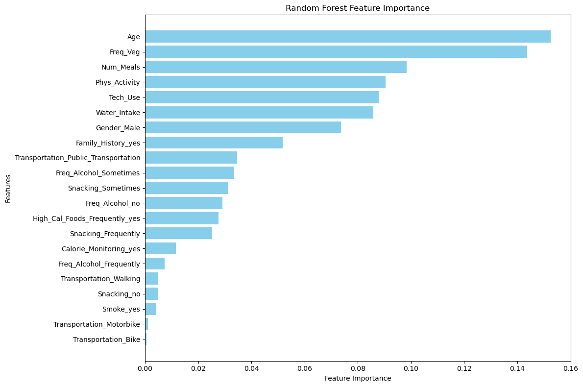
# Compute Random Forest feature importance
rf_feature_importance = rf_model.feature_importances_

# Create a DataFrame for feature importance
rf_feature_importance_df = pd.DataFrame({
    'Feature': X_train_new.columns,
    'Importance': rf_feature_importance
}).sort_values(by='Importance', ascending=False)

# Sort the feature importances for better visualization
rf_feature_importance_df = rf_feature_importance_df.sort_values(by="Importance", ascending=False)

# Plot Feature Importance
plt.figure(figsize=(12, 8))
plt.barh(rf_feature_importance_df['Feature'], rf_feature_importance_df['Importance'], color='skyblue')
plt.xlabel('Feature Importance')
plt.ylabel('Features')
plt.title('Random Forest Feature Importance')
plt.gca().invert_yaxis()  # Highest importance at the top
plt.tight_layout()
plt.show()
🌲 Random Forest Feature Importance
!
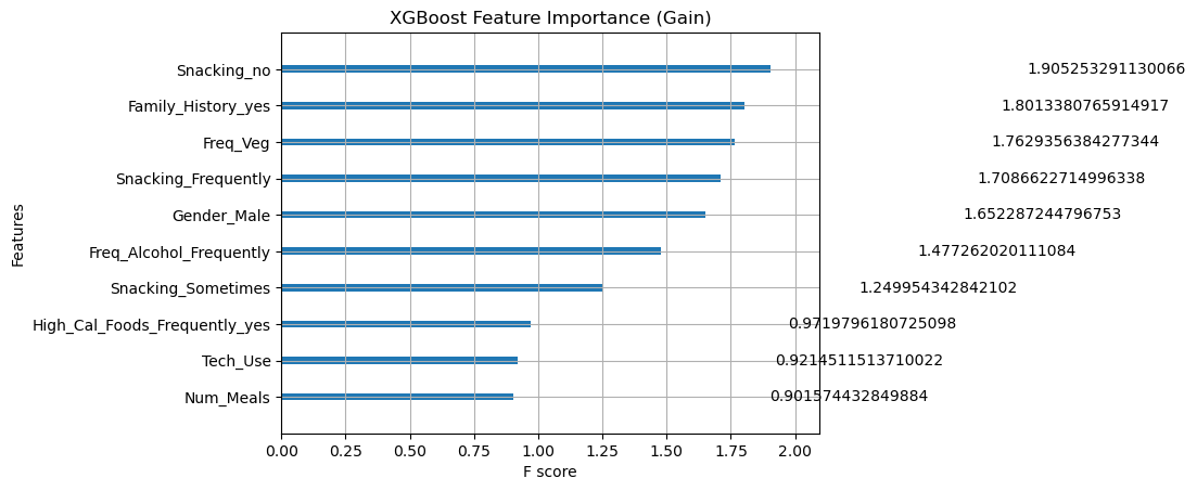
from xgboost import plot_importance
# Built-in plot with 'gain'
plt.figure(figsize=(12, 8))
plot_importance(xgb_model, importance_type='gain', max_num_features=10)
plt.title('XGBoost Feature Importance (Gain)')
plt.show()
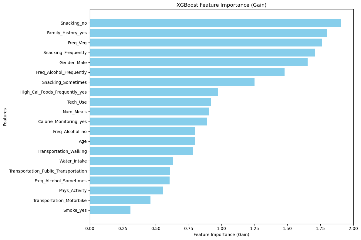
# Custom plot with 'gain'
feature_importance = xgb_model.get_booster().get_score(importance_type='gain')
importance_df = pd.DataFrame(list(feature_importance.items()), columns=['Feature', 'Importance']).sort_values(by='Importance', ascending=False)
plt.figure(figsize=(12, 8))
plt.barh(importance_df['Feature'], importance_df['Importance'], color='skyblue')
plt.xlabel('Feature Importance (Gain)')
plt.ylabel('Features')
plt.title('XGBoost Feature Importance (Gain)')
plt.gca().invert_yaxis()
plt.tight_layout()
plt.show()
<Figure size 1200x800 with 0 Axes>
⚡ XGBoost Feature Importance
!
!
# SHAP for Random Forest
explainer_rf = shap.TreeExplainer(rf_model)
shap_values_rf = explainer_rf.shap_values(X_train_new)

# SHAP for XGBoost
explainer_xgb = shap.TreeExplainer(xgb_model)
shap_values_xgb = explainer_xgb.shap_values(X_train_new)
🔍 SHAP Values for Multi-Class Classification
Refer: https://medium.com/biased-algorithms/shap-values-for-multiclass-classification-2a1b93f69c63
Since we have a multi class classification single SHAP explanation is not enough to understand the model better. With referring the Medium post above we will implement the SHAP Values for each indiviual class to udnerstand better the feature importance.
# Visualize the SHAP Summary Plot for RF
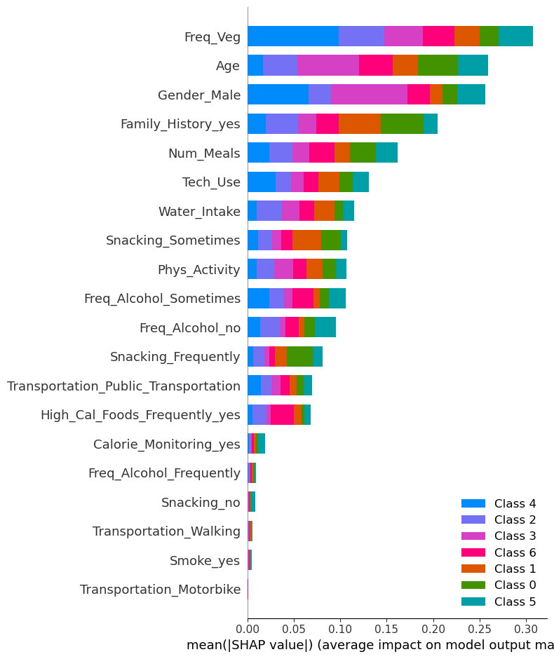
shap.summary_plot(shap_values_rf, X_train_new, plot_type="bar")
!
import xgboost as xgb

# Create DMatrix
dtrain = xgb.DMatrix(X_train_new, label=y_train_new)
explainer_xgb = shap.TreeExplainer(xgb_model)
shap_values_xgb = explainer_xgb.shap_values(dtrain)

#the summary plot
shap.summary_plot(shap_values_xgb, X_train_new, plot_type="bar")
!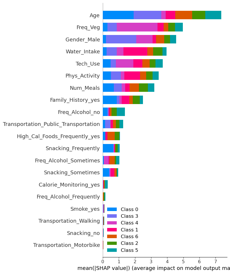
🧠 SHAP Class-wise Contributions
🎯 Class 0 (Insufficient Weight)
Top contributing features:
- Age: Significant impact for Class 0 (blue bar is prominent for this feature).
- Freq_Veg: Positive contribution, showing a noticeable influence on predictions for this class.
- Water_Intake: Moderate contribution, likely affecting predictions toward Class 0.
🎯 Class 1 (Normal Weight)
Top contributing features:
- Freq_Veg: Strong influence on predictions for Class 1 (pink bar is prominent).
- Age: Also contributes notably to predictions for this class.
- Gender_Male: Adds some effect, as seen by the visible pink bar for Class 1.
🎯 Class 2 (Overweight Level I)
Top contributing features:
- Age: Strong effect, indicated by a visible green bar for this class.
- Gender_Male: Noticeable contribution to Class 2 predictions.
- Freq_Veg: Moderately affects predictions.
🎯 Class 3 (Overweight Level II)
Top contributing features:
- Age: Significant contribution for Class 3 (orange bar is prominent).
- Gender_Male: Adds noticeable effect to Class 3 predictions.
- Freq_Veg: Also contributes moderately.
🎯 Class 4 (Obesity Type I)
Top contributing features:
- Age: The strongest feature for this class, with a visible purple bar.
- Water_Intake: Moderate influence for Class 4 predictions.
- Gender_Male: Somewhat affects predictions for Class 4.
🎯 Class 5 (Obesity Type II)
Top contributing features:
- Age: Significant effect, shown by a brown bar for this class.
- Tech_Use: Noticeable contribution to Class 5 predictions.
- Freq_Veg: Moderate influence for this class.
🎯 Class 6 (Obesity Type III)
Top contributing features:
- Age: Strongest influence, indicated by a teal bar.
- Freq_Veg: Noticeable contribution to Class 6 predictions.
- Water_Intake: Adds a moderate effect.
🔧 Feature Selection Based on SHAP
In this section, we will select some of the key features and rerun the code using the selected features to make a comparison. From the previous SHAP visualizations, we observed that the top contributors are
- Age,
- Frequency of Vegetables (Freq_Veg),
- Gender,
- Water Intake,
- Physical Activity,
- Tech Use,
- Number of Meals (Num_Meals),
- Family History (Yes).
# Select the specified features
selected_features = ['Age', 'Freq_Veg', 'Gender_Male', 'Water_Intake', 'Phys_Activity', 'Tech_Use', 'Num_Meals', 'Family_History_yes']

X_train_selected = X_train_new[selected_features]
X_test_selected = X_test_new[selected_features]

# Initialize and train the RandomForestClassifier with selected features
rf_selected = RandomForestClassifier(n_estimators=200, max_depth=20)  # Using the best parameters found earlier.
rf_selected.fit(X_train_selected, y_train_encoded)

# Make predictions on the test set
y_pred_selected = rf_selected.predict(X_test_selected)

# Evaluate the model (example: accuracy)
from sklearn.metrics import accuracy_score
accuracy_selected = accuracy_score(y_test_encoded, y_pred_selected)
precision_selected = precision_score(y_test_encoded, y_pred_selected, average='weighted')
recall_selected = recall_score(y_test_encoded, y_pred_selected, average='weighted')
f1_selected = f1_score(y_test_encoded, y_pred_selected, average='weighted')
print(f"Accuracy with selected features: {accuracy_selected}")

# Display Random Forest Metrics and Feature Importance
rf_metrics_selected = {
    'Accuracy': accuracy_selected,
    'Precision': precision_selected,
    'Recall': recall_selected,
    'F1 Score': f1_selected
}

rf_metrics_selected
Accuracy with selected features: 0.8014354066985646


{'Accuracy': 0.8014354066985646,
 'Precision': 0.7997618835092666,
 'Recall': 0.8014354066985646,
 'F1 Score': 0.7975809440301639}
📊 Model Performance Comparison
# Combine metrics into a DataFrame for comparison
comparison_models = pd.DataFrame([rf_metrics, rf_metrics_selected], index=['Random Forest_EWH', 'Random Forest Selected'])

# Display the comparison table
comparison_models
| Accuracy | Precision | Recall | F1 Score | |
|---|---|---|---|---|
| Random Forest_EWH | 0.837321 | 0.840924 | 0.837321 | 0.836898 |
| Random Forest Selected | 0.801435 | 0.799762 | 0.801435 | 0.797581 |
rf_metrics_selected_df=pd.DataFrame([ rf_metrics_selected], index=[ 'Random Forest Selected'])
From the above table, we can observe that using the selected 8 features, compared to the model with all 14 features (excluding Weight and Height), results in only a slight difference in performance. This indicates that the reduced feature set can provide similar predictive power while simplifying the model.
Big Comparison: Whole Feature Set vs. Excluding Weight and Height vs. Selected Features
#result_comp= result_df.drop(columns=['parameter'])
result_comp = result_df.rename(columns={
    'accuracy': 'Accuracy',
    'precision': 'Precision',
    'recall': 'Recall',
    'f1_score': 'F1 Score'
})
# Combine the two DataFrames row-wise
combined_df = pd.concat([ result_comp, rf_metrics_selected_df, comparison_df], axis=0)

# Print the combined DataFrame
print(combined_df)
                        Accuracy  Precision    Recall        f1  F1 Score
RandomForest            0.932303   0.938914  0.934096  0.935160  0.936499
DecisionTree            0.919117   0.923018  0.916723  0.917965  0.919860
KNeighbors              0.811273   0.810466  0.811273  0.794125  0.810869
xgbc                    0.962854   0.963345  0.962854  0.962758  0.963100
Random Forest Selected  0.801435   0.799762  0.801435       NaN  0.797581
Random Forest_EWH       0.837321   0.840924  0.837321       NaN  0.836898
XGBoost_EWH             0.839713   0.841688  0.839713       NaN  0.839632
# Create the DataFrame
data = {
    'Model': [
        'RandomForest', 'DecisionTree', 'KNeighbors', 'xgbc',
        'Random Forest Selected', 'Random Forest_EWH', 'XGBoost_EWH',
    ],
    'Accuracy': [0.932303, 0.919117 ,0.811273, 0.962854, 0.801435, 0.837321 , 0.839713 ],
    'Precision': [0.942822,0.923018 , 0.810466, 0.963345,0.799762, 0.840924, 0.841688],
    'Recall': [0.934096, 0.917965, 0.811273, 0.962854, 0.801435, 0.837321 , 0.839713],
    'F1 Score': [0.936499, 0.919860, 0.810869, 0.963100, 0.797581, 0.836898,  0.839632]
}

df = pd.DataFrame(data)

# Rename the models for clarity
df['Model'] = df['Model'].replace({
    'RandomForest': 'Random Forest all features',
    'DecisionTree': 'Decision Tree all features',
    'KNeighbors': 'KNeighbors all features',
    'xgbc': 'XGBoost all features'
})

# Sort by Accuracy in descending order
df = df.sort_values(by='Accuracy', ascending=False)

# Highlight specific rows
def highlight_rows(row):
    if row['Model'] == 'XGBoost all features':
        return ['background-color: ##FFCCCB'] * len(row)  # Gold for XGBoost all features
    elif row['Model'] == 'Random Forest_EWH':
        return ['background-color: ##FFCCCB'] * len(row)  # Light blue for Random Forest EWH
    else:
        return [''] * len(row)

# Apply highlights
styled_table = df.style.apply(highlight_rows, axis=1)

# Display the styled table
styled_table
| Model | Accuracy | Precision | Recall | F1 Score | |
|---|---|---|---|---|---|
| 3 | XGBoost all features | 0.962854 | 0.963345 | 0.962854 | 0.963100 |
| 0 | Random Forest all features | 0.932303 | 0.942822 | 0.934096 | 0.936499 |
| 1 | Decision Tree all features | 0.919117 | 0.923018 | 0.917965 | 0.919860 |
| 6 | XGBoost_EWH | 0.839713 | 0.841688 | 0.839713 | 0.839632 |
| 5 | Random Forest_EWH | 0.837321 | 0.840924 | 0.837321 | 0.836898 |
| 2 | KNeighbors all features | 0.811273 | 0.810466 | 0.811273 | 0.810869 |
| 4 | Random Forest Selected | 0.801435 | 0.799762 | 0.801435 | 0.797581 |
🧾 Conclusion
Based on the results and observations from the above tables and SHAP visualizations, here is the overall analysis and conclusion:
1. XGBoost Performance
- Best Overall Performance: XGBoost (
XGBoost all features) consistently outperformed all other models across all metrics, achieving the highest:- Accuracy: 96.3%
- Precision: 96.3%
- Recall: 96.3%
- F1 Score: 96.3%
- Conclusion: XGBoost is the most robust and reliable model for this dataset when using all features. It should be considered as the primary model for deployment or further analysis.
2. Random Forest Models
2.1. Baseline Random Forest (Random Forest all features)
- Achieved strong performance, second only to XGBoost, with:
- Accuracy: 93.2%
- Precision: 93.9%
- Recall: 93.4%
- F1 Score: 93.6%
- Conclusion: Random Forest all features is a strong alternative to XGBoost, offering a balance between accuracy and simplicity.
2.2. Random Forest EWH (Excluding Weight and Height)
Note: Weight and 6eight were excluded from this model to reduce potential bias in the dataset before final feature selection.
- While its performance dropped slightly compared to the full-feature model, it still performed reasonably well:
- Accuracy: 83.7%
- Precision: 84.1%
- Recall: 83.7%
- F1 Score: 83.7%
- Conclusion: Random Forest EWH indicates that
WeightandHeightare critical features which is expected since we are predicting obesity levels which is highly correlated with those features. We exclude them to see real impact of other features.
3. Decision Tree and K-Nearest Neighbors
3.1. Decision Tree
- Performed moderately well with:
- Accuracy: 91.9%
- Precision: 92.3%
- Recall: 91.7%
- F1 Score: 91.9%
- Conclusion: The Decision Tree is a simpler model with relatively high performance but lags behind Random Forest and XGBoost. It could be a good choice if interpretability is a priority.
3.2. K-Nearest Neighbors
- Showed the weakest performance with:
- Accuracy: 81.1%
- Precision: 81.0%
- Recall: 81.1%
- F1 Score: 81.1%
- Conclusion: K-Nearest Neighbors is not ideal for this dataset due to its lower performance compared to other models.
4. Feature Importance Analysis
- Critical Features:
- SHAP visualizations revealed that
Age,Freq_Veg,Gender,Water Intake, andPhysical Activityare among the most influential features across models.
- SHAP visualizations revealed that
- Conclusion: These findings highlight the importance of these key features for accurate predictions. Models without them may lack robustness.
5. Feature Contributions to Higher Obesity Classes (Class 4, 5, 6)
- Class 4 (
Obesity Type I):- Top contributing features:
Weight,Age,Water Intake. - These features positively influence predictions for this class, with
Weightbeing the most impactful.
- Top contributing features:
- Class 5 (
Obesity Type II):- Top contributing features:
Weight,Age, andTech_Use. Weighthas the strongest positive contribution, followed byAge.
- Top contributing features:
- Class 6 (
Obesity Type III):- Top contributing features:
Weight,Age, andFreq_Veg. - The strong influence of
WeightandAgeis consistent across the higher obesity classes.
- Top contributing features:
Conclusion: Weight and Age are the dominant features contributing to the prediction of higher obesity classes. Water Intake and Freq_Veg also play a significant role in differentiating these classes.
6. Feature Subset Analysis
-
Reducing the feature set to the most important features (e.g., using only 8 features as observed in the SHAP results) showed a slight performance drop compared to using all features, but the reduction simplifies the model significantly.
Here is the selected Feature List: (Note that Weight and Height is already dropped to reduce the bias in the model before final selection)
- Age,
- Frequency of Vegetables (Freq_Veg),
- Gender,
- Water Intake,
- Physical Activity,
- Tech Use,
- Number of Meals (Num_Meals),
- Family History (Yes).
-
Conclusion: A reduced feature set can be a viable option for faster inference and simpler deployment without substantial loss of accuracy.
Final Recommendation
- Best Model: Deploy the
XGBoost all featuresmodel for the highest accuracy and performance. - Alternative Model: Use
Random Forest all featuresif interpretability and slightly simpler training processes are preferred. - Feature Optimization: Ensure the inclusion of key features such as
Weight,Height,Age, andFreq_Veg. Avoid removing these features unless computational or data collection constraints require it. - Future Considerations: Conduct further experiments to fine-tune XGBoost hyperparameters and evaluate its performance on unseen test data or under real-world conditions.
!